# Deconvolution with RCTD
# Visium HD spatial transcriptomics workshop
# Author: Harvard Chan Bioinformatics Core
# Created: May 2026
# Load libraries
library(Seurat)
library(tidyverse)
library(spacexr) # Contains RCTD function
# Set parallelization (multithreading) to speed up calculations
plan("multicore", workers = parallel::detectCores() - 1)
# Increases the size of the default vector (8GB)
options(future.globals.maxSize = 8000 * 1024^2)
# Load dataset
seurat_banksy <- readRDS("data/intermediate_seurat/seurat_banksy.rds")Deconvolution
Spatial transcriptomics
Deconvolution
Cell type annotation
This lesson breaks down multi-cell spatial spots into estimated cell type proportions using deconvolution methods such as RCTD with single-cell RNA-seq references. This lesson covers reference preparation, model fitting and visualization of cell composition across tissue.
Keywords
RCTD, scRNA-seq, Cell proportions
Approximate time: 40 minutes
Learning objectives
In this lesson, we will:
- Load and investigate our reference dataset used for cell type annotation
- Convert our Seurat object into an RCTD data structure
- Deconvolve bins to assign cell types and assess the annotation
Overview of lesson
While the clusters are helpful in identifying groups of bins that are similar to one another, we have not yet determined the cell type for each bin. For sequencing-based methods, deconvolution is a great first step in determining the cell type for each spot, given that a bin may have multiple cells contained within it. We will be using the method Robust Cell Type Deconvolution (RCTD) to assign cell type labels for each bin. These deconvolution outputs are reused in subsequent analyses, such as cell–cell communication.
What is deconvolution?
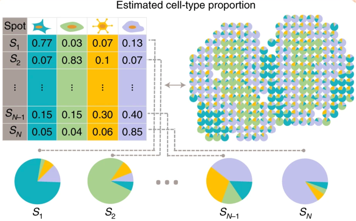
The single-digit micron resolution is a big technological improvement over Visium’s original ∼55μm spots. Because a single spot could include several cell types, the dataset is not straightforward to annotate. As a result, many methods model each spot as a mixture, assigning proportion values for each cell type within that spot. Each spot is represented as a piechart showing proportions of the cell type composition.
While Visium HD reduces bin size to approach single-cell resolution, it is important to note that this sequencing-based spatial transcriptomics captures RNA from a defined spatial area rather than from isolated cells. As a result, transcripts from multiple cells overlapping in a bin would be pooled and sequenced together. This means that even small bins may contain mixed cellular signals, which has important implications for downstream analyses, such as differential gene expression.
Imaging-based technologies
It is important to note that up until this point, the entire workflow we have been using would work for either imaging- or sequencing-based spatial technologies. Deconvolution is not an appropriate step for imaging-based technologies.
This is because when we work with imaging-based technologies, we are using single-cells after segmentation. Therefore it does not make sense to model a mixture of cell types when the input is single cells. As a result, the annotation for these datasets follows a similar workflow as celltyping a single-cell experiment.
To annotate your dataset, we recommend to do a mixture of the following:
- Use marker genes from the literature that are specific to a cell type
- Identify top genes per cluster to map cell types to clusters
- Apply automatic celltyping algorithms (i.e Azimuth, CellTypist, SingleR, etc.)
Robust Cell Type Deconvolution (RCTD)
We will carry out our deconvolution in a new script called 06_deconvolution.R, which will be kept in our scripts directory. At the top of the script, we will add a header, call our libraries and load our Seurat object.
To perform accurate annotation of cell types, we must also take into consideration that our 8µm x 8µm bins may contain multiple cells. The method Robust Cell Type Deconvolution (RCTD) has been shown to accurately annotate spatial datasets from a variety of technologies, while taking into consideration that a single bin may exhibit multiple cell type profiles.
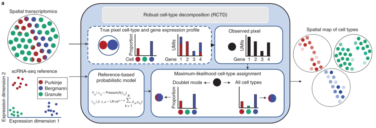
Image source: Cable et al., 2021
The overarching process of RCTD involves several steps:
- RCTD calculates the average gene expression for each cell type in a reference single-cell RNA sequencing dataset.
- Each bin/pixel in the query spatial transcriptomics data is treated as containing an unknown mix of multiple cell types.
- RCTD fits each pixel as a combination of different cell types, where each cell type contributes a proportion of the gene counts observed.
- For each pixel and gene, the observed gene counts are assumed to follow a Poisson distribution in the probability model.
- Estimates for cell type proportions in each pixel are calculated with a maximum-likelihood estimate (MLE).
- Lastly, RCTD can be run in two ways:
- Standard mode: no limit on the number of cell types per pixel.
- Doublet mode: restricts each pixel to a maximum of one or two cell types.
RCTD uses an annotated scRNA-seq dataset (reference) and our spatial dataset (query) as input. Creating these objects will be the first step of this analysis.
Reference dataset
For our reference, we will use the paired scRNA-seq FLEX dataset that was generated from the same patients as the original study. The code for how this object was created can be found here.
First, let us load in the reference Seurat object that we downloaded with the spatial dataset at the beginning of the workshop.
# Load Seurat reference dataset
seurat_ref <- readRDS("data/crc_flex_ref_downsample.RDS")
seurat_refAn object of class Seurat
18082 features across 4500 samples within 1 assay
Active assay: RNA (18082 features, 0 variable features)
1 layer present: counts
1 dimensional reduction calculated: umapWe can take a look at the unique cell types in the reference dataset by plotting the UMAP of the reference dataset. These are stored in column Level1 and should give us a better understanding of the make-up of our dataset by cell type.
# Set idents
Idents(seurat_ref) <- "Level1"
# UMAP of reference dataset
p <- DimPlot(seurat_ref) +
ggtitle("RCTD Reference Dataset")
# Add cluster labels
LabelClusters(p,
id = "ident",
fontface = "bold",
size = 3,
bg.colour = "white",
bg.r = .2,
force = 0)
Running RCTD
As mentioned earlier, there are two main inputs that must be supplied to RCTD:
- Reference: an object containing the raw counts and cell type column in metadata.
- Query: a spatial transcriptomics object that we want to deconvolve against the reference.
We are going to create some custom RCTD objects out of our original Seurat object for RCTD. This will essentially create a new data structure that fits with what the Run.RCTD() function expects.
Create reference
Now that we better understand the reference, we are going to make an RCTD object out of it. We will use the Reference() function to cast our Seurat object into the correct format. We supply the following three parameters:
counts= raw counts matrixcell_types= cell type annotationnUMI= total number of counts per cell (nCount)
# Raw counts of reference dataset
counts <- seurat_ref[["RNA"]]$counts
# cell type annotation of reference dataset (must be a factor)
cluster <- seurat_ref$Level1
cluster <- as.factor(cluster)
# Total counts of each cell
nUMI <- seurat_ref$nCount_RNA
# Create the RCTD reference object
reference <- Reference(counts = counts,
cell_types = cluster,
nUMI = nUMI)
Structure of
reference
When we look at the structure of this reference object, we can see that we have our nUMI, counts and cell_types in this object.
str(reference)Formal class 'Reference' [package "spacexr"] with 3 slots
..@ cell_types: Factor w/ 9 levels "B cells","Endothelial",..: 9 9 8 8 2 9 5 2 8 4 ...
.. ..- attr(*, "names")= chr [1:4500] "AAAGGTGAGTCACCTAACTTTAGG-1" "AACTGAATCCTGGAAGACTTTAGG-1" "AAGGCACGTTCTTGAAACTTTAGG-1" "AAGGCTGTCGGTACGAACTTTAGG-1" ...
..@ counts :Formal class 'dgCMatrix' [package "Matrix"] with 6 slots
.. .. ..@ i : int [1:4460158] 112 136 174 194 226 227 240 277 292 303 ...
.. .. ..@ p : int [1:4501] 0 748 3659 4860 5210 5996 6923 7425 9815 10501 ...
.. .. ..@ Dim : int [1:2] 18082 4500
.. .. ..@ Dimnames:List of 2
.. .. .. ..$ : chr [1:18082] "SAMD11" "NOC2L" "KLHL17" "PLEKHN1" ...
.. .. .. ..$ : chr [1:4500] "AAAGGTGAGTCACCTAACTTTAGG-1" "AACTGAATCCTGGAAGACTTTAGG-1" "AAGGCACGTTCTTGAAACTTTAGG-1" "AAGGCTGTCGGTACGAACTTTAGG-1" ...
.. .. ..@ x : num [1:4460158] 2 1 1 1 1 1 1 1 2 1 ...
.. .. ..@ factors : list()
..@ nUMI : Named num [1:4500] 936 4725 1542 407 1078 ...
.. ..- attr(*, "names")= chr [1:4500] "AAAGGTGAGTCACCTAACTTTAGG-1" "AACTGAATCCTGGAAGACTTTAGG-1" "AAGGCACGTTCTTGAAACTTTAGG-1" "AAGGCTGTCGGTACGAACTTTAGG-1" ...Create query
Deconvolution is very computationally expensive! So we can once again make use the sketch workflow to downsample our dataset in a careful manner. Additionally, we are going to split our Seurat object into a single sample P5CRC. There are extensions of the RCTD package in order to take into account replicates and multiple samples which we will not use at this time due to time constraints.
# Subset to P5CRC sample
crc <- subset(seurat_banksy,
subset = (orig.ident == "P5CRC"))
# Inspect the Seurat object
crcAn object of class Seurat
36170 features across 57463 samples within 2 assays
Active assay: Spatial.008um (18085 features, 2000 variable features)
2 layers present: counts, data
1 other assay present: sketch
6 dimensional reductions calculated: pca.sketch, umap.sketch, full.pca.sketch, full.umap.sketch, pca.banksy, harmony.banksy
1 spatial field of view present: P5CRC.008umWe cannot use the same sketch information from the previous lessons since this is one sample (and not both). Therefore, we are going to quickly run through the sketch workflow one more time. However, we will not be running the entire workflow, as we only need the PCA scores to project back to the larger dataset.
# Create sketch of CRC subset
# Set default assay
DefaultAssay(crc) <- 'Spatial.008um'
# HVGs are required input for SketchData
crc <- FindVariableFeatures(object = crc,
assay = "Spatial.008um")
# Calculate leverage score
crc <- SketchData(
object = crc,
ncells = 5000,
method = "LeverageScore",
sketched.assay = "sketch_crc",
var.name = "leverage.score_crc")
# Run through processing workflow
# Stop at PCA
crc <- FindVariableFeatures(crc)
crc <- ScaleData(crc)
crc <- RunPCA(crc,
reduction.name = "pca.sketch_crc")RCTD requires another unique data structure as input to run. So we will create our query object with SpatialRNA() by suppling the spatial coordinates and raw counts for the bins. Note that we do not have to supply any cell type information, like we did with the reference object earlier. This is because we don’t have any cell type information yet! That is the output we are hoping to generate from running RCTD.
# Get raw counts of downsampled sketch assay
DefaultAssay(crc) <- "sketch_crc"
counts_sketch <- crc[["sketch_crc"]]$counts
# Grab barcodes for sketched bins
cells_sketch <- colnames(crc[["sketch_crc"]])
# Spatial coordinates for each bin in sketch assay
coords <- GetTissueCoordinates(crc)[cells_sketch, c("x", "y")]
# Grab nUMI per sketch bin
nUMI_sketch <- crc@meta.data[cells_sketch, "nCounts_Spatial.008um"]
# Create the RCTD query object
query <- SpatialRNA(coords = coords,
counts = counts_sketch,
nUMI = nUMI_sketch)
Structure of
query
When we look at the structure of this query object, we can see that we have our nUMI, counts and coords in this object.
str(query)Formal class 'SpatialRNA' [package "spacexr"] with 3 slots
..@ coords:'data.frame': 5000 obs. of 2 variables:
.. ..$ x: num [1:5000] 60621 54093 53817 56712 56687 ...
.. ..$ y: num [1:5000] 62512 58219 61315 60684 59866 ...
..@ counts:Formal class 'dgCMatrix' [package "Matrix"] with 6 slots
.. .. ..@ i : int [1:2337095] 13 90 174 261 377 677 904 1012 1027 1133 ...
.. .. ..@ p : int [1:5001] 0 121 496 1523 2012 2224 2692 3347 3903 4218 ...
.. .. ..@ Dim : int [1:2] 18085 5000
.. .. ..@ Dimnames:List of 2
.. .. .. ..$ : chr [1:18085] "SAMD11" "NOC2L" "KLHL17" "PLEKHN1" ...
.. .. .. ..$ : chr [1:5000] "P5CRC_s_008um_00052_00559-1" "P5CRC_s_008um_00198_00335-1" "P5CRC_s_008um_00092_00326-1" "P5CRC_s_008um_00114_00425-1" ...
.. .. ..@ x : num [1:2337095] 1 1 1 1 1 1 1 1 1 2 ...
.. .. ..@ factors : list()
..@ nUMI : Named num [1:5000] 128 503 1576 750 238 ...
.. ..- attr(*, "names")= chr [1:5000] "P5CRC_s_008um_00052_00559-1" "P5CRC_s_008um_00198_00335-1" "P5CRC_s_008um_00092_00326-1" "P5CRC_s_008um_00114_00425-1" ...Run RCTD
Now that we have created our reference and query objects, we will create an RCTD object and use thee run.RCTD() function. This should take 5-10 minutes to run.
# Set-up for RCTD run by supplying both query and reference
RCTD <- create.RCTD(spatialRNA = query,
reference = reference,
max_cores = parallel::detectCores() - 1)
# Run deconvolution
# This step may take 5-10 minutes to run
RCTD <- run.RCTD(RCTD, doublet_mode = "doublet")Note that RCTD can take longer when you have more cell types, which is the reason we used the Level1 annotation of cell types over Level2 from the reference dataset.
RCTD results
The resulting dataframe from RCTD will contain the following columns according to the documentation:
| Column | Description |
|---|---|
spot_class |
RCTD’s classification (doublet mode): • singlet – 1 cell type on pixel• doublet_certain – 2 cell types on pixel• doublet_uncertain – 2 cell types on pixel, but only confident of 1• reject – no prediction given for pixel |
first_type |
First cell type predicted on the bin; defined for all spot_class values except reject. |
second_type |
Second cell type predicted on the bin for doublet spot_class (doublet_certain, doublet_uncertain); not a confident prediction in the doublet_uncertain case. |
The results of deconvolution are stored in the results$results_df slot of the RCTD object:
# Grab results dataframe and view first few rows
df_rctd_results <- RCTD@results$results_df
df_rctd_results %>%
head()| spot_class | first_type | second_type | first_class | second_class | min_score | singlet_score | conv_all | conv_doublet | |
|---|---|---|---|---|---|---|---|---|---|
| P5CRC_s_008um_00052_00559-1 | singlet | Myeloid | Endothelial | FALSE | FALSE | 247.6690 | 248.6940 | TRUE | TRUE |
| P5CRC_s_008um_00198_00335-1 | singlet | Tumor | Intestinal Epithelial | FALSE | FALSE | 412.7892 | 414.9878 | TRUE | TRUE |
| P5CRC_s_008um_00092_00326-1 | singlet | Tumor | Intestinal Epithelial | FALSE | FALSE | 873.5261 | 874.7588 | TRUE | TRUE |
| P5CRC_s_008um_00114_00425-1 | singlet | Intestinal Epithelial | B cells | FALSE | FALSE | 595.2669 | 595.0713 | TRUE | TRUE |
| P5CRC_s_008um_00142_00424-1 | singlet | Endothelial | Fibroblast | FALSE | FALSE | 347.1421 | 350.3347 | TRUE | TRUE |
| P5CRC_s_008um_00131_00541-1 | singlet | Intestinal Epithelial | Tumor | FALSE | FALSE | 550.9241 | 557.3652 | TRUE | TRUE |
We can also visualize the number of identifications established for each first_type:
# Number of cell types annotated to each bin in sketch assay
ggplot(df_rctd_results,
aes(x = first_type,
fill = first_type)) +
geom_bar() +
theme_bw() + NoLegend() +
ggtitle("P5CRC: RCTD First Type Results") +
theme(axis.text.x = element_text(angle = 90,
vjust = 0.5,
hjust=1))
Just by looking at the total number of bins, this is a good reminder that we only have the RCTD results for the 5,000 bins we sketched to.
Project RCTD results on all bins
Let us take a look at how many rows (bins) we have these annotations for:
nrow(df_rctd_results)[1] 4809But didn’t our sketch assay include 5,000 bins? RCTD runs its own QC step that filters out bins with low expression or rejects bins where it is unable to map a cell type from the reference dataset. This is why we have fewer bins than we expected. So we are going to do some data wrangling to ensure that we keep track of all information. Including those ~200 bins without first_type labels. In a future step, we will set the label for these bins to be unassigned.
To do so, we are first going to do some wrangling to the results dataframe:
- Append
_sketchto all column names - Remove factors (to avoid downstream errors)
# Update column names to have _sketch
# Add "sketch" to column names
colnames(df_rctd_results) <- paste0(colnames(df_rctd_results),
"_sketch")
# Create column "cell" to merge on
# Removing factors for easier merging later
df_rctd_results <- df_rctd_results %>%
mutate(cell = rownames(df_rctd_results)) %>%
mutate(first_type_sketch = as.character(first_type_sketch),
second_type_sketch = as.character(second_type_sketch),
spot_class_sketch = as.character(spot_class_sketch))
# Make sure columns were generated
colnames(df_rctd_results) [1] "spot_class_sketch" "first_type_sketch" "second_type_sketch"
[4] "first_class_sketch" "second_class_sketch" "min_score_sketch"
[7] "singlet_score_sketch" "conv_all_sketch" "conv_doublet_sketch"
[10] "cell" Now, let us merge this information into our Seurat object. This step is necessary because in order to ProjectData(), we need the RCTD results to live in our @meta.data slot.
# Create cell barcode in metadata
crc$cell <- rownames(crc@meta.data)
meta <- crc@meta.data
# Merge together RCTD results and metadata
meta <- left_join(x = meta,
y = df_rctd_results,
by = "cell")
rownames(meta) <- meta$cell
# Put meta into crc Seurat object
crc@meta.data <- metaProject back to full dataset
Now, we can run the ProjectData(), just like we did last time in order to project out RCTD results to the full CRC dataset.
# Project back first_type to new column called first_type
# This will fail
crc <- ProjectData(
object = crc,
assay = "Spatial.008um",
sketched.assay = "sketch_crc",
full.reduction = "pca_crc",
sketched.reduction = "pca.sketch_crc",
dims = 1:30,
refdata = list(spot_class = "spot_class_sketch",
first_type = "first_type_sketch",
second_type = "second_type_sketch"))Error in `TransferLablesNN()`:
! wrong weights matrix inputWhy did we get an error when we tried to get RCTD labels for the entire dataset? This is because we have those NA values for bins in the sketch assay. The ProjectData() function expects actual values for every sketched bin. Therefore, to get around this issue, we are going to label those bins as unassigned in the metadata.
# Set value of unassigned to sketch bins that do not have values
# This is because ProjectData will throw errors otherwise
cols <- c("spot_class_sketch",
"first_type_sketch",
"second_type_sketch")
# Iterate through each column to set "unassigned" to NA values
for (col in cols) {
# Find rows that are in sketch_cells and are NA
na_rows <- cells_sketch[is.na(crc@meta.data[cells_sketch, col])]
# Assign the value to unassigned
crc@meta.data[na_rows, col] <- "unassigned"
}
Number of unassigned bins
We can use the table() function to quickly see how many unassigned bins we have in our dataset:
# Show the number of bins assigned to each cell type, including unassigned
table(crc@meta.data$first_type_sketch)
B cells Endothelial Fibroblast
387 326 413
Intestinal Epithelial Myeloid Neuronal
1462 420 91
Smooth Muscle T cells Tumor
127 247 1336
unassigned
191 At this point, we have assigned labels for each bin in the sketch assay. So we can once again run ProjectData() and this time get cell type labels for each bin in our dataset.
# Project back first_type to new column called first_type
crc <- ProjectData(
object = crc,
assay = "Spatial.008um",
sketched.assay = "sketch_crc",
full.reduction = "pca_crc",
sketched.reduction = "pca.sketch_crc",
dims = 1:30,
refdata = list(spot_class = "spot_class_sketch",
first_type = "first_type_sketch",
second_type = "second_type_sketch"))Visualize RCTD results
Now that we have first_type values associated with each bin, we can visualize our dataset in a variety of different ways.
Barplot
We can get an overview of how many bins we have with a barplot. As we might expect, the number of unassigned bins increased as we extrapolate the labels out to the larger dataset.
# Barplot of first_type labels after ProjectData()
ggplot(crc@meta.data,
aes(x = first_type, fill = first_type)) +
geom_bar() +
theme_bw() + NoLegend() +
ggtitle("P5CRC: Projected First Type RCTD") +
theme(axis.text.x = element_text(angle = 90, vjust = 0.5, hjust=1))
ProjectData().
This visual primes us to expect that the majority of the bins in our dataset are intestinal epithelial cells. From the original publication, we also know that these epithelial cells can be broken down even further into goblet and enterocytes (from Level2 annotation of the reference dataset).
Spatial overlay
We can also see how the bins are located on the slide itself.
# Spatial plot of first_type labels after ProjectData()
SpatialDimPlot(crc,
group.by = "first_type",
pt.size.factor = 15,
image.alpha = 0.5)
ProjectData().
Alternative spatial visualization
Sometimes it can be difficult to see patterns for a given cell type when all of the cell types are present in the same plot. Due to this difficulty, we can also facet our different cell types into their own plots:
# Grab x, y coordinates and first_type cell type labels
df <- FetchData(crc,
vars = c("x", "y",
"first_type"))
# Create scatterplot
ggplot(df,
aes(x = x, y = y,
color = first_type)) +
geom_point(size = 0.05) +
theme_bw() +
# Split by cell type label
facet_wrap(~first_type) +
NoLegend()
ProjectData() split by first_type.
As we previously noted, the left-most region on th P5CRC slide is comprised primarily of tumor cells. There are some myeloid and fibroblast cells mixed throughout this region as well. The rest of the tissue contains mostly epithelial cells, which is to be expected when we consider the layered structure of the colon.
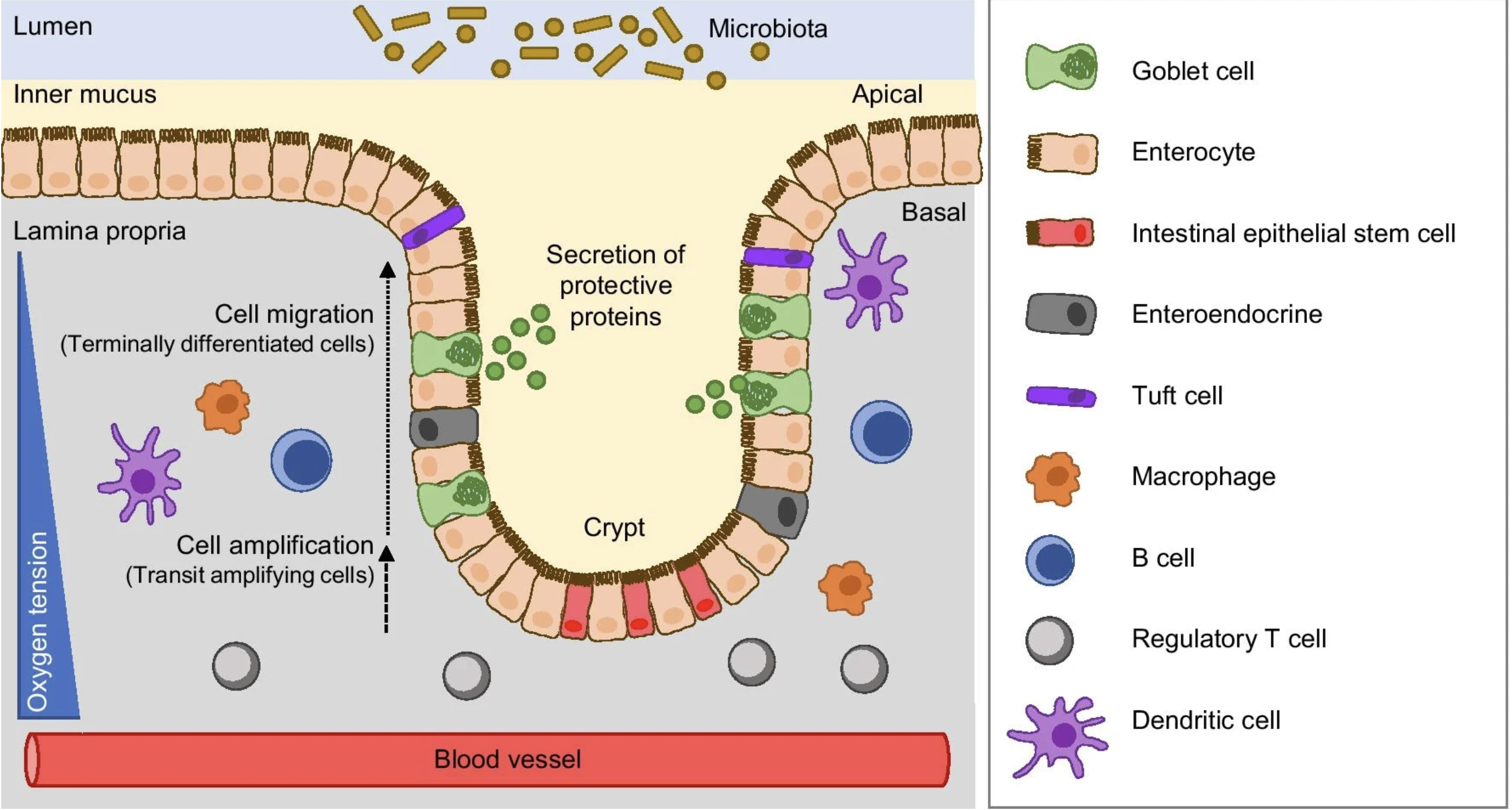
Image source: Ternet et al. (2021)
The colon wall is organized into distinct layers. The innermost surface facing the gut cavity is lined by epithelial cells (goblet, enterocyte, tuft cells), which form a structure known as Crypts of Lieberkühn. These cells form a barrier, selectively allowing interactions between the gut microbiome and the inner regions of the tissue (mucosa). Here, the immune component (T and B cells) are present. Right underneath there is another layer of muscle cells, known as the muscularis mucosae, which is responsible for the folded structure of the colon. Together, these layers allow the colon to control what passes from the gut cavity into the rest of the tissue.
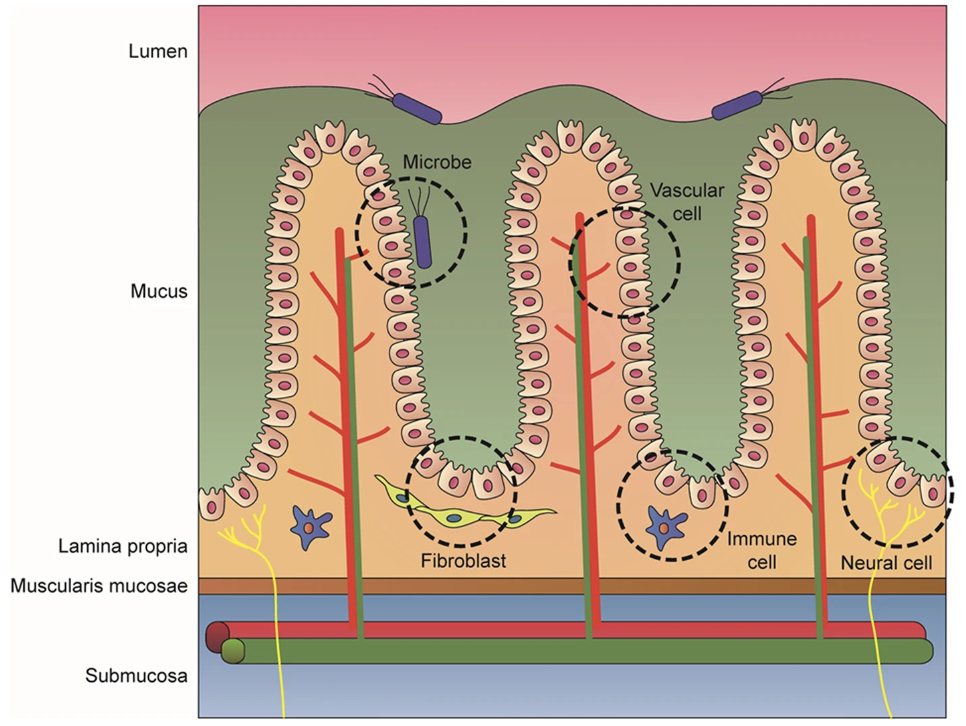
Image source: Min et al. (2020)
This is consistent with what we observe in our own dataset, where the immune cells (B and T cells) are found deeper within the tissue rather than at the surface. Recall that this is the P5CRC sample, meaning that the structure will not be exactly as shown in these schematics due to the abnormalities caused by cancer. In the P5NAT sample, we will be able to more clearly see the normal colon structure outlined here.
UMAP
We can now see how the cell types fall on our UMAP space.
# UMAP of reference dataset
Idents(crc) <- "first_type"
p <- DimPlot(crc,
reduction = "full.umap.sketch") +
ggtitle("P5CRC RCTD First Type")
LabelClusters(p, id = "ident", fontface = "bold", size = 3,
bg.colour = "white", bg.r = .2, force = 0)
ProjectData().
As we might expect, the immune populations (myeloid, T and B cells) appear close to one another in UMAP space due to the similarity of their gene expression. The most distinctly clustered populations are the tumor and epithelial bins, which have very different gene expression patterns compared to the rest of the cell types in the dataset.
P5CRC and P5NAT results
We have run RCTD of the full dataset for both P5CRC and P5NAT for you all to load and run the rest of the workshop with:
# Load Seurat object with P5CRC and P5NAT cell type annotations
seurat_rctd <- readRDS("data/intermediate_seurat/seurat_RCTD.rds")# Spatial plot of first_type labels after ProjectData()
SpatialDimPlot(seurat_rctd,
group.by = "first_type",
pt.size.factor = 15,
image.alpha = 0)
ProjectData() for both samples.
What is the sample-specific proportion for each
first_type? Create a ggplot barplot showing the proportions of each cell type. Hint: Refer back to the code we used here.Create a dotplot using the known marker genes for each cell type to see if the
first_typelabels align with known cell type genes.
marker_list <- list(
"B cells" = c("IGKC", "IGHM", "CD79A", "MS4A1", "MZB1"),
"Endothelial cells" = c("PECAM1", "VWF", "PLVAP", "ENG", "KLF2"),
"Fibroblasts" = c("COL1A1", "COL3A1", "DCN", "LUM", "COL6A2"),
"Intestinal epithelial cells" = c("CLCA1", "FCGBP", "MUC2", "PIGR", "ZG16"),
"Myeloid cells" = c("C1QC", "SELENOP", "SPP1", "LYZ", "CD68"),
"Neural cells" = c("NRXN1", "L1CAM", "NCAM1", "VIP", "CALB2"),
"Smooth muscle cells" = c("TAGLN", "ACTA2", "MYH11", "MYL9", "CNN1"),
"T cells" = c("TRAC", "CD3E", "TRBC2", "IL7R", "CD52"),
"Tumor cells" = c("CEACAM6", "CEACAM5", "EPCAM", "KRT8", "LCN2")
)Do we generally agree with the annotation that was done with RCTD based upon these results?
Reuse
CC-BY-4.0