# Moran's I
# Visium HD spatial transcriptomics workshop
# Author: Harvard Chan Bioinformatics Core
# Created: May 2026
# Load libraries
library(tidyverse)
library(Seurat)
set.seed(12345)
# Increases the size of the default vector (8GB)
options(future.globals.maxSize = 8000 * 1024^2)
# Set parallelization (multithreading) to speed up calculations
library(future)
plan(multisession, workers = parallel::detectCores() - 1)
# Load dataset
seurat_rctd <- readRDS("data/intermediate_seurat/seurat_RCTD.rds")Spatially Variable Genes
Spatial transcriptomics
SVGs
Moran's $I$
In this lesson, we will identify spatially variable genes (SVGs) whose expression changes across tissue locations. This lesson shows how to detect, visualize and prioritize SVGs as markers of spatial domains and gradients.
Keywords
Variable genes, Spatial patterns, Spatial autocorrelation, Spatial gradients
Approximate time: 30 minutes
Learning objectives
In this lesson, we will:
- Define the Moran’s \(I\) calculation
- Run Moran’s \(I\) to identify spatially variable genes
- Visualize spatially variable genes
Overview of lesson
At this step, instead of comparing defined cell types, you might ask which genes vary as a function of spatial location. In this lesson we will apply methods for detecting spatially variable genes (SVGs), then map and visualize their expression patterns across the tissue. These genes often serve as interpretable anchors for defining domains, building signatures and linking expression to morphology.
Spatially variable genes (SVGs)
Spatially variable genes (SVGs) are similar in concept to highly variable genes (HVGs). HVGs were identified by evaluating the variability of gene expression across the entire dataset. However, now we have the additional layer of the spatial location for each bin. As a result, we are able to identify genes that have different levels of expression depending on which area of the tissue they are found in.
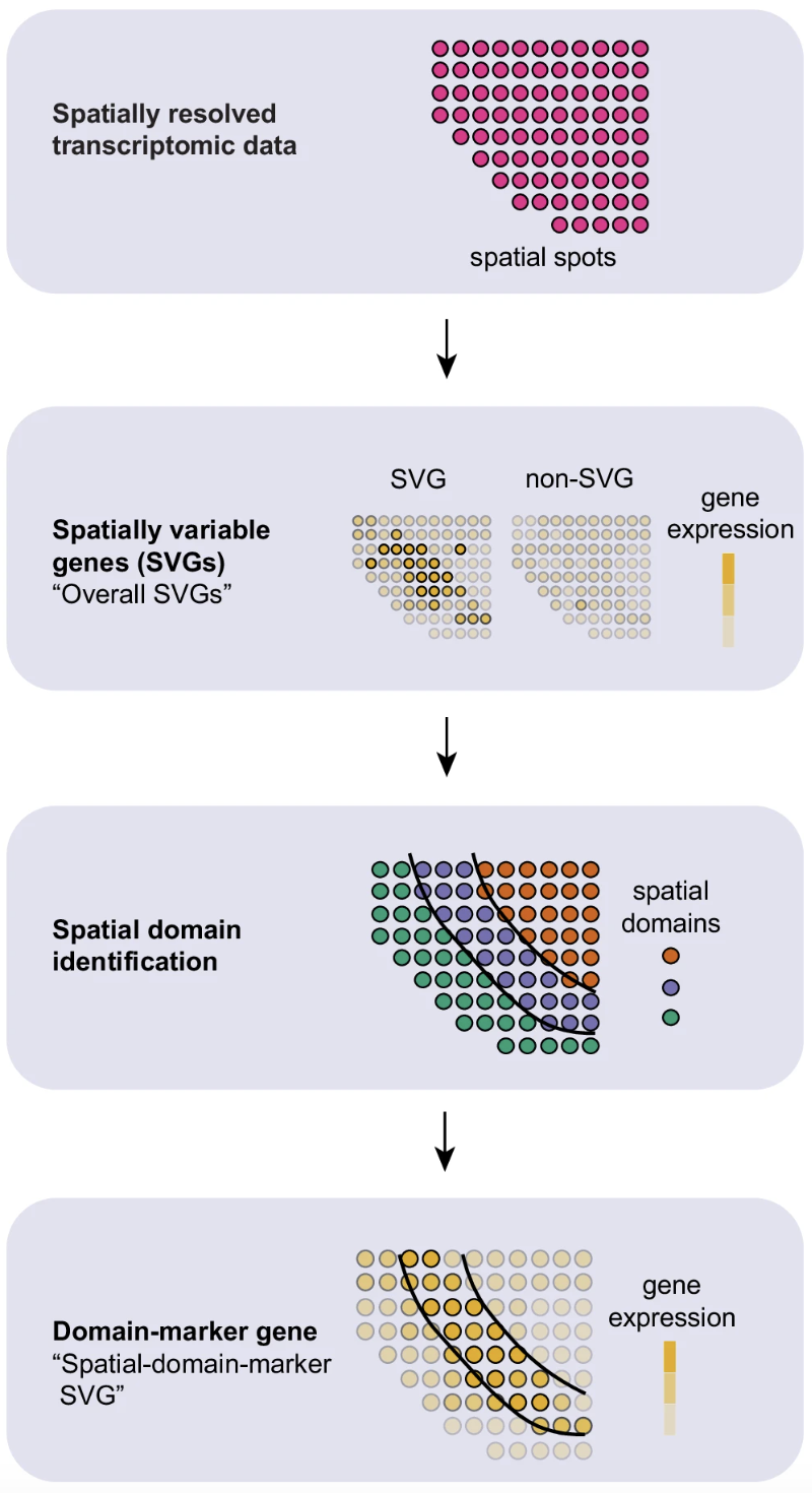
Image source: Yan et al., 2025
These methods can be used to identify genes that have strong spatial associations for downstream analyses - similar to how we used HVGs to calculate PCA. These SVGs can also be used to evaluate spatial niches within cell-types to assist in finding subtypes within the tissue.
Ultimately, these genes provide another peek into the spatial context of the tissue.
Moran’s \(I\)
Many of the SVG algorithms are built upon the concept of Moran’s \(I\), which is defined as “a measure of spatial autocorrelation”. The math behind the method is defined like so:
\[ I = \frac{N}{S_0} \frac{ \sum_{i=1}^N \sum_{j=1}^N w_{ij}\,(x_i - \bar{x})(x_j - \bar{x}) }{ \sum_{i=1}^N (x_i - \bar{x})^2 } \]
where:
- \(N\) is the number of spatial units, indexed by \(i\) and \(j\);
- \(x\) is the variable of interest;
- \(\bar{x}\) is the mean of \(x\);
- \(w_{ij}\) are the elements of the spatial-weights matrix, with \(w_{ii} = 0\);
- \(S_0\) is the sum of all spatial weights, \(S_0 = \sum_{i=1}^N \sum_{j=1}^N w_{ij}\).
Breakdown of Moran’s \(I\) calculation
In simpler terms, the Moran’s \(I\) calculation looks at two bins at a time, \(i\) and \(j\). The term \(w_{ij}\) is a measure of “closeness” between bins \(i\) and \(j\), where greater influence (weight) is given to bins that are spatially near to one another.
This calculation is done one gene at a time, so we get an \(I\) value for each gene, represented as \(x\) in the equation. Here, \(\bar{x}\) is the average expression of a gene across all bins in the dataset. When we calculate \((x_i - \bar{x})\) and \((x_j - \bar{x})\), we are subtracting the normalized expression of gene \(x\) for bins \(i\) and \(j\) from the average expression. In essence, we are calculating the deviation from the mean for both bins. This calculation is run for every pair of bins in the dataset, with the weighted products being summed together.
Additionally, we normalize the score in the denominator by calculating the gene’s variance with \(\sum_{i=1}^N (x_i - \bar{x})^2\) in the dataset. The last component of the equation is to multiply \(\frac{N}{S_0}\) to the results. This is to scale the final \(I\) value in such a way that we can compare results from different genes against one another, even if there are different spatial weights and gene expression distributions.
The range of values for Moran’s \(I\) E(I) in spatial transcriptomics is usually [-1, 1].
For a random spatial distribution, Moran’s \(I\) will be near zero. A large positive value indicates the data is clustered. A large negative value indicates that the data is dispersed, meaning units that are close spatially have dissimilar variable values.
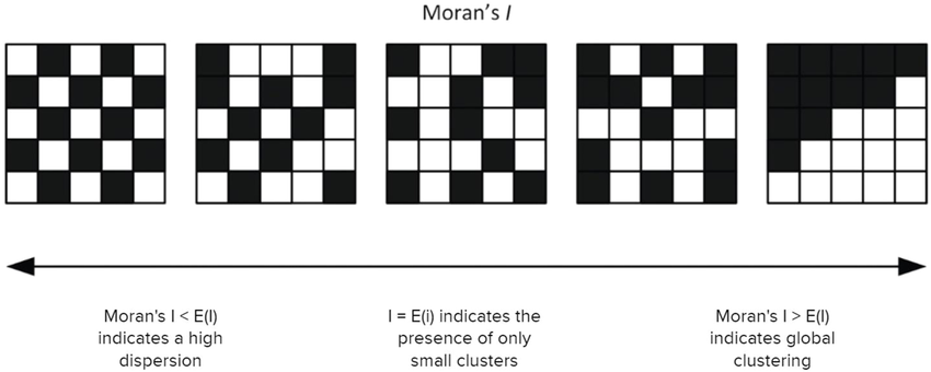
Image source: Tsui et al., 2022
To see why this is the case, consider the expression \((x_i - \bar{x}) (x_j - \bar{x})\) in the above formula. If \(x_i\) and \(x_j\) are similar and far from the mean, then this product will be large and positive. If they are dissimilar (in particular, if one is well above the mean and one is far below) then this product will be large and negative. If \(x_i\) and \(x_j\) are both similar to the mean, then this value would be small. Note that Moran’s \(I\) depends strongly on the calculation of \(w_{ij}\), which represents the spatial relations of the bins. A large value \(w_{ij}\) indicates that bins \(i\) and \(j\) are close spatially.
Running Moran’s \(I\)
Moran’s \(I\) will work best if we focus on one sample at a time, as the spatial coordinates will be consistent within a single slide. Furthermore, because this step can take a long time to run, we are going to further subset the data to a singular cell type. In this way, we are attempting to evaluate genes that are specific to spatially defined subtype of a cell type.
Let’s begin by creating a new R script, 08_SVGs.R, and adding it to our scripts directory:
For this example, let us zoom in on the tumor cells in the CRC dataset:
# Subset to tumor P5CRC bins
crc_sub <- subset(seurat_rctd,
subset = (orig.ident == "P5CRC") &
(first_type == "Tumor"))
crc_subAn object of class Seurat
36170 features across 12855 samples within 2 assays
Active assay: Spatial.008um (18085 features, 2000 variable features)
2 layers present: counts, data
1 other assay present: sketch
6 dimensional reductions calculated: pca.sketch, umap.sketch, full.pca.sketch, full.umap.sketch, pca.banksy, harmony.banksy
1 spatial field of view present: P5CRC.008umFor the best results, we are going to make use of the scale.data assay (this is typically calculated right before the PCA step). We only ever calculated this on the sketch assay, so here we will run the ScaleData() function on our entire subsetted dataset.
# Re-calculate HVGs on subset data
crc_sub <- FindVariableFeatures(crc_sub)
# Scale log-normalized counts
crc_sub <- ScaleData(crc_sub)
crc_subAn object of class Seurat
36170 features across 12855 samples within 2 assays
Active assay: Spatial.008um (18085 features, 2000 variable features)
3 layers present: counts, data, scale.data
1 other assay present: sketch
6 dimensional reductions calculated: pca.sketch, umap.sketch, full.pca.sketch, full.umap.sketch, pca.banksy, harmony.banksy
1 spatial field of view present: P5CRC.008umWe can now calculate Moran’s \(I\) with the FindSpatiallyVariableFeatures() function and set the selection.method = "moransi". We are additionally going to specify that we want to evaluate Moran’s \(I\) on the top 50 highly variable genes. A gene that is spatially variable is likely to also be highly variable because ultimately we are assessing changes in gene expression across different populations. We take the top 50 to reduce the number of calculations that take place (so we can reasonably run this on a laptop). Ideally you would run this on the full set of highly variable genes.
This step may take a few minutes to run.
# Run Moran's I on the top 50 highly variable genes
crc_sub <- FindSpatiallyVariableFeatures(crc_sub,
selection.method = "moransi",
verbose = TRUE,
features = VariableFeatures(crc_sub)[1:50],
image = "P5CRC.008um")Once the calculation completes, we can evaluate the Moran’s \(I\) scores and associated p-values for each of the genes. We will have to do a bit of subsetting as we only calculated these values for 50 genes.
# Moran's I scores for each gene
SVFInfo(crc_sub, method = "moransi") %>%
subset(!is.na(MoransI_observed)) %>%
arrange(desc(MoransI_observed)) %>%
head()FindSpatiallyVariableFeatures() with associated Moran’s \(I\) scores and p-values.
| MoransI_observed | MoransI_p.value | |
|---|---|---|
| PIGR | 0.5056012 | 0.0009756 |
| REG3A | 0.4772619 | 0.0009756 |
| OLFM4 | 0.4213175 | 0.0009756 |
| PI3 | 0.3579835 | 0.0009756 |
| MUC17 | 0.2544224 | 0.0009756 |
| PPBP | 0.2205412 | 0.0009756 |
Then, we can use the SpatiallyVariableFeatures() function to get the list of SVGs that were just calculated. For visualization purposes, we are going to grab the top 10 genes.
# Get top 10 spatially variable features
top10_svg <- SpatiallyVariableFeatures(crc_sub,
method = "moransi")
top10_svg <- top10_svg[1:10]
top10_svg [1] "PIGR" "REG3A" "OLFM4" "PI3" "MUC17" "PPBP" "SULT1C4"
[8] "CHGB" "IGHG1" "CHGA" And visualize the expression of these genes on the spatial slide:
# Spatial plot of top SVGs
SpatialFeaturePlot(crc_sub,
features = top10_svg[1:6],
pt.size.factor = 15,
image.alpha = 0.1,
ncol = 3)
Notice that all of these genes have noticeable patterns of expression that are constrained to specific regions of the tissue. This is the power of spatially variable genes! We can identify genes where there is a clear spatial component to their expression patterns.
Recall in the BANKSY lesson we noted that the BANKSY algorithm identified different, spatially constrained subtypes in this cancerous region. For example, we can zoom in clusters 13, 14, and 15.
# Grab x and y coordinates for plotting
# Also get the sample ID and the banksy cluster score for each bin
df <- FetchData(crc_sub,
vars = c("x", "y",
"banksy_cluster"))
# Subset to one sample (P5CRC)
ggplot(df %>% subset(banksy_cluster %in% c(13, 14, 15)),
# Plot spatial coordinates and color by cluster
aes(x = x, y = -y,
color = banksy_cluster)) +
geom_point(size = 0.05) +
theme_bw() +
# Create separate plots for each cluster
facet_wrap(~banksy_cluster) +
NoLegend()
Interestingly, clusters 14 and 15 appear to be associated with the top and bottom of the tissue. This suggests that there is a spatial organization of cells with different function.
So now we can begin to see which of those genes were defining the phenotype of these tumor subtypes.
# Dotplot of tumor clusters for top SVGs
DotPlot(crc_sub,
top10_svg,
group.by = "banksy_cluster",
cluster.idents = TRUE,
idents = c(13, 14, 15)) +
theme(axis.text.x = element_text(angle = 45, hjust = 1))
A distinct phenotype emerges for each group of cancerous regions.
For instance, cluster 14 shows strong expression of OLFM4, a known marker of intestinal stem cells and tumor cells typically located at the base of epithelial crypts. These cells differentiate into secretory lineages, resembling Paneth cells, which are not usually present in the colon. Furthermore, this differentiation is associated with reduced cell adhesion capabilities.
In contrast, cluster 15 is characterized by high expression of REG3A, which plays a key role in modulating gut microbiome interactions by killing Gram-positive bacteria. Increased REG3A expression has been reported in multiple cancer types and is typically associated with enhanced proliferation of endocrine cells.
We can see that while both clusters 14 and 15 are tumor cells, they differ both spatially and in gene expression. Meanwhile, cluster 13 appears to be a transient state between the two populations. Using spatially variable genes, we can start defining regions of the tissue and annotate the function of those regions. This will help us understand the spatial organization of the tissue.
- Pick a different cell type and run
FindSpatiallyVariableFeatures(). Name the population you chose and print the top 6 genes in the results.
SVG use cases and methods
There are many different use cases of these SVGs, for example:
- Instead of HVGs as input for PCA, use SVGs to run the workflow all the way to clustering
- Identify spatial regions based upon top SVGs (e.g cortical layers)
- Classify subtypes of broader cell types
As the field of spatial transcriptomics is ever evolving, there are other algorithms that utilize different priors to identify spatially variable genes. Some methods include, but are not limited to:
Note that some of these are written in Python.
Reuse
CC-BY-4.0