# CellChat
# Visium HD spatial transcriptomics workshop
# Author: Harvard Chan Bioinformatics Core
# Created: May 2025
# Load libararies
library(tidyverse)
library(Seurat)
library(CellChat)
set.seed(12345)
# Increases the size of the default vector (8GB)
options(future.globals.maxSize = 8000 * 1024^2)
# Set parallelization (multithreading) to speed up calculations
library(future)
plan(multisession, workers = parallel::detectCores() - 1)
# Load dataset
seurat_rctd <- readRDS("data/intermediate_seurat/seurat_RCTD.rds")CellChat
Spatial transcriptomics
Cell-cell communication
CellChat
Ligand-receptor analysis
In this lesson, we will analyze cell–cell communication in spatial transcriptomics using CellChat to infer signaling networks. You will build interaction graphs between celltypes and relate spatial proximity to signaling strength.
Keywords
Ligands, Receptors, Interaction graph, Signaling strength
Approximate time: 60 minutes
Learning objectives
In this lesson, we will:
- Create a CellChat object
- Run the CellChat workflow to calculate ligand-receptor interactions
- Visualize ligand receptor interactions
Overview of lesson
At this point in our analysis, we are comfortable with the celltype annotations of our dataset. So we might start asking questions about how each of those populations are interacting with one another. In this lesson, we will use CellChat to build directed signaling networks. These interaction maps help connect static expression patterns to dynamic biological processes such as immune infiltration, niche signaling or tumor–stroma crosstalk.
Cell-cell communication
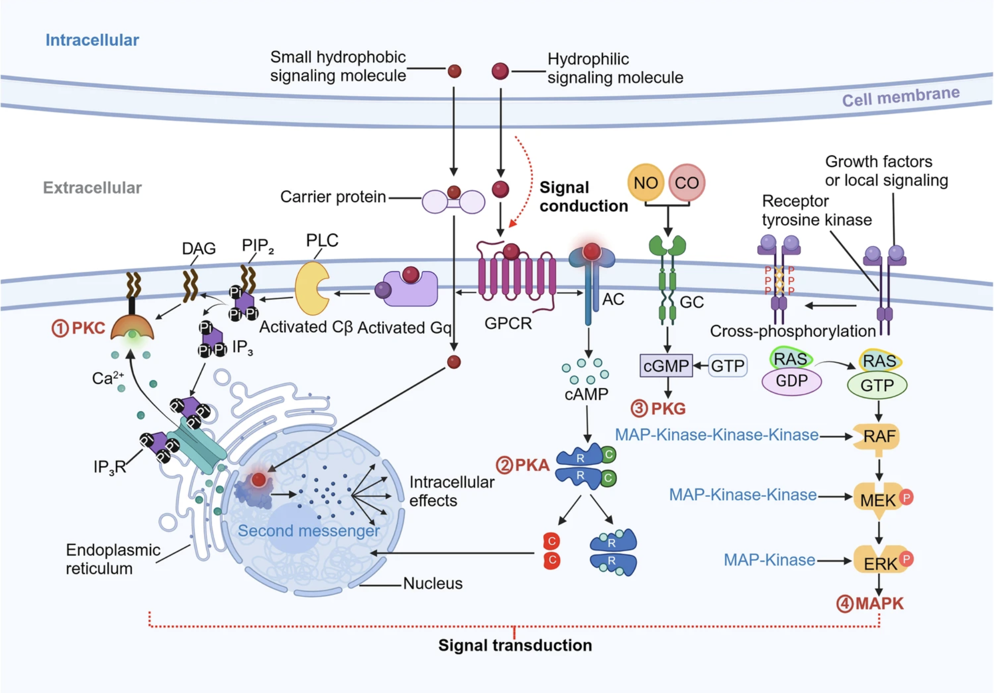
Image source: Su et al., 2024
We know that cells do not exist in an isolated environment, where they do not interact with anything. The opposite is true, where cells interact with one another and exchange information through various mechanisms, such as signal transduction for activating proteins. Understanding which cells interact with each other is crucial for understanding how cell differentiation, organ development and metabolism is modulated.
Spatial transcriptomics is a great input dataset for these methods because cell interactions are oftentimes between cells in close proximity. The coordinates become a powerful input parameter to improve the accuracy of interaction results.
CellChat
CellChat is a method that was originally published by Jin et al., 2021, and then updated several years later Jin et al., 2025, to incorporate spatial coordinates into the model. The outputs of CellChat are lists of significant ligand-receptor interactions between cell types.
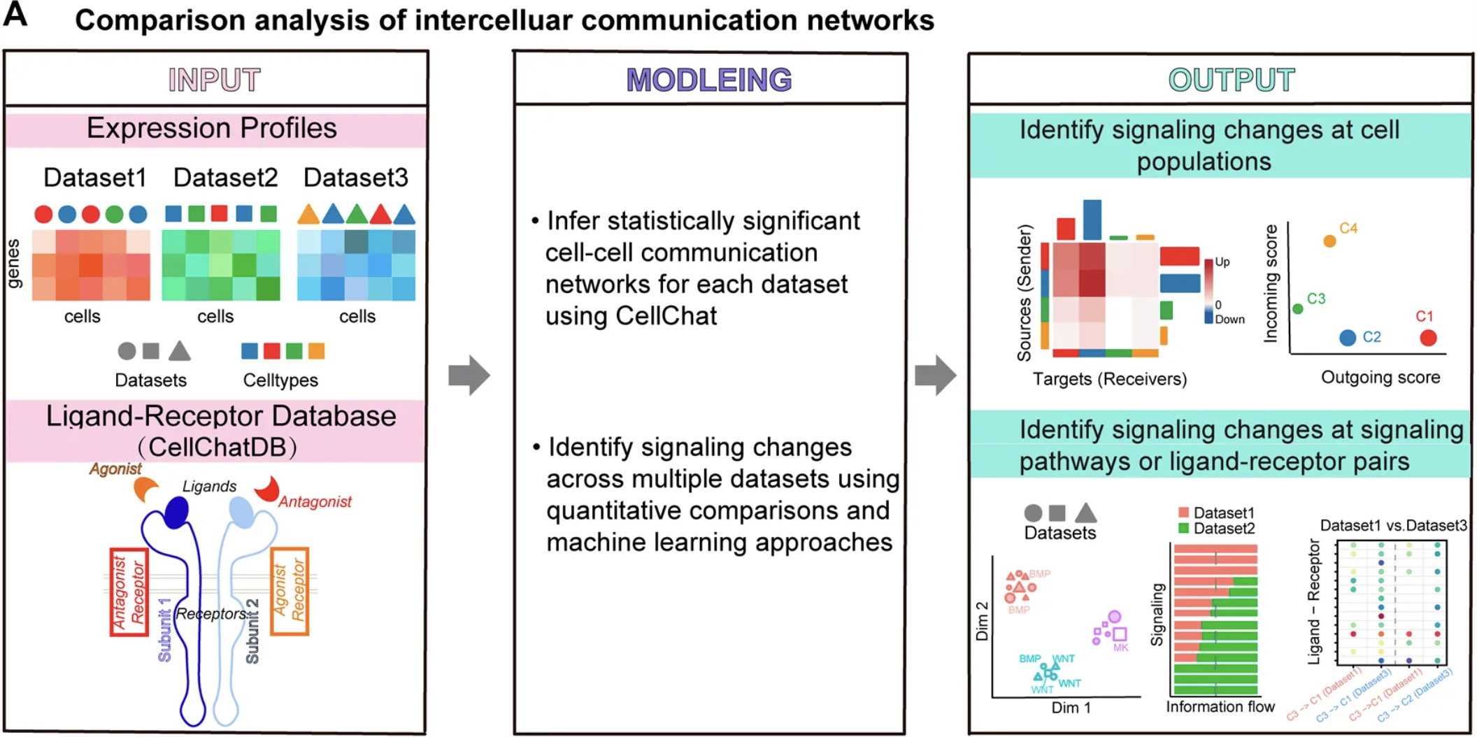
Image source: Hao et al., 2021
First, the authors created a database of known ligand-receptor interactions from the literature classified as: secreted signaling, extracellular matrix recepotrs and cell-cell contact. This database is used in conjunction with your own dataset and its celltype labels to identify communcations between populations. In essence, the method identifies overexpressed ligand receptors from the database in your own data to measure association using the principle of mass action. Using this assumption, if there is high expression of a ligand in a cell type and high expression of a receptor, then the probability of ligand-receptor interaction strength is high.
Running cellchat
CellChat was written such that you run the workflow on one sample at a time and then merge all datasets together to run a comparative analysis. So here, we are going to focus on the ligand-receptor results for our P5CRC dataset. As this is a new analysis, we will create a new script titled 09_cellchat.R and place it within our scripts directory:
For now, let us say that our biological question is to identify which populations are interacting with the tumor cells in colorectal cancer. So first, we are going to subset the Seurat object to our relevant bins.
# Subset to CRC sample
# Remove unassigned bins
crc <- subset(seurat_rctd,
subset = (orig.ident == "P5CRC") &
(first_type != "unassigned"))
# CellChat expects a "samples" column that is a factor
crc$samples <- factor(crc$orig.ident)
crcAn object of class Seurat
36170 features across 53017 samples within 2 assays
Active assay: Spatial.008um (18085 features, 2000 variable features)
2 layers present: counts, data
1 other assay present: sketch
6 dimensional reductions calculated: pca.sketch, umap.sketch, full.pca.sketch, full.umap.sketch, pca.banksy, harmony.banksy
1 spatial field of view present: P5CRC.008umCreate CellChat object
Similar to RCTD, CellChat has its own data structure for storing information. In order to create this object with the createCellChat() function, we must provide the following pieces of information:
object: Normalized counts matrixcoordinates: Spatial coordinates for each binspatial.factors: Spatial factors (stored in json file)
To generate these, we can use the GetAssayData() to grab the log-normalized counts from the crc Seurat object:
# Get normalized counts matrices
counts_norm_crc <- GetAssayData(crc,
assay = "Spatial.008um",
layer = "data")
counts_norm_crc[1:5, 1:5]| P5CRC_s_008um_00128_00278-1 | P5CRC_s_008um_00052_00559-1 | P5CRC_s_008um_00121_00413-1 | P5CRC_s_008um_00202_00633-1 | P5CRC_s_008um_00035_00460-1 | |
|---|---|---|---|---|---|
| SAMD11 | 0 | 0 | 0 | 0 | 0 |
| NOC2L | 0 | 0 | 0 | 0 | 0 |
| KLHL17 | 0 | 0 | 0 | 0 | 0 |
| PLEKHN1 | 0 | 0 | 0 | 0 | 0 |
| PERM1 | 0 | 0 | 0 | 0 | 0 |
Next, we will grab the spatial coordinates associated with each bin. Here, we will use the FetchData() function to grab the coordinates we stored in the @meta.data. You could also use the ouput from the GetTissueCoordinates() function as well.
# Get spatial coordinates
coords_crc <- FetchData(crc, vars = c("x", "y"))
coords_crc %>% head()| x | y | |
|---|---|---|
| P5CRC_s_008um_00128_00278-1 | 52418.69 | 60257.61 |
| P5CRC_s_008um_00052_00559-1 | 60620.61 | 62512.22 |
| P5CRC_s_008um_00121_00413-1 | 56362.64 | 60478.41 |
| P5CRC_s_008um_00202_00633-1 | 62800.98 | 58138.03 |
| P5CRC_s_008um_00035_00460-1 | 57725.67 | 62997.04 |
| P5CRC_s_008um_00126_00342-1 | 54288.57 | 60323.76 |
We now need to grab the spatial.factors which is described as a dataframe with ratio and tol, where:
ratio: conversion from image units (e.g., pixels) to micrometers. For example:ratio = 0.18means1 pixel = 0.18 µm.tol: distance tolerance to make center-to-center distance comparisons more robust, often set to about half the cell/spot size (in µm).
Luckily, these values are stored in the scalefactors_json.json file that Space Ranger outputs. So we will need to load in the file using jsonlite and then create a dataframe with the relevant information.
# Scale factors stored in Space Ranger json output file
sf_json <- jsonlite::fromJSON("data/P5CRC_cropped/binned_outputs/square_008um/spatial/scalefactors_json.json")
# Create spatial.factors dataframe
spatial_factors_crc <- data.frame(
# Pixels-to-µm conversion factor
ratio = sf_json$bin_size_um / sf_json$spot_diameter_fullres,
# Neighbour tolerance radius in µm
tol = sf_json$bin_size_um / 2)
spatial_factors_crc ratio tol
1 0.2736934 4With all three input files needed for createCellChat() generated, we can start the CellChat workflow. We will additionally supply our metadata as well as the column which contains our cell type annotations (first_type).
# Create cellchat object
cellchat_crc <- createCellChat(
object = counts_norm_crc,
coordinates = coords_crc,
spatial.factors = spatial_factors_crc,
meta = crc@meta.data,
group.by = "first_type",
datatype = "spatial")[1] "Create a CellChat object from a data matrix"
Create a CellChat object from spatial transcriptomics data...
Set cell identities for the new CellChat object
The cell groups used for CellChat analysis are B cells, Endothelial, Fibroblast, Intestinal Epithelial, Myeloid, Neuronal, Smooth Muscle, T cells, Tumor # Display the CellChat object
cellchat_crcAn object of class CellChat created from a single dataset
18085 genes.
53017 cells.
CellChat analysis of spatial data! The input spatial locations are
x_cent y_cent
P5CRC_s_008um_00128_00278-1 52418.69 60257.61
P5CRC_s_008um_00052_00559-1 60620.61 62512.22
P5CRC_s_008um_00121_00413-1 56362.64 60478.41
P5CRC_s_008um_00202_00633-1 62800.98 58138.03
P5CRC_s_008um_00035_00460-1 57725.67 62997.04
P5CRC_s_008um_00126_00342-1 54288.57 60323.76CellChat databset
CellChatDB is the database that contains the manually curated set of ligand-receptor interactions created by the authors. It includes the following types of interactions:
- Secretory autocrine/paracrine signaling interactions
- Cell-cell contact interactions
- Extracellular matrix (ECM)-receptor interactions
- Non-protein signaling
We want to incorporate this information into our cellchat_crc so that when we run CellChat, the workflow will automatically know which interactions to include in the analysis. This database is available for both mouse and human. Since we are working with human samples, we will use CellChatDB.human and we assign this to our CellChat object.
# Load CellChat databases
cellchat_db <- CellChatDB.human
# Assign DB to cellchat object in the DB slot
cellchat_crc@DB <- cellchat_db
Subset CellChatDB
The database contains ligand-receptors that can be broadly categorized in 4 groups:
# Pie chart of cellchat database categories
showDatabaseCategory(cellchat_db)
If you are only interested in a particular group of interactions, say from one on the signaling groups, you can use the subsetDB() function and specificy which group you want in the search argument.
Here we show what the full list of categories are:
# DO NOT RUN
# Subset CellChatDB for cell-cell communication analysis
cellchat_db <- subsetDB(cellchat_db,
search = c("Secreted Signaling",
"ECM-Receptor",
"Cell-Cell Contact",
"Non-protein Signaling"))Now that the database is linked to our dataset, we need to run the subsetData() function to filter the dataset to the signaling genes to save on computation.
# Subset step is required even if you have not filtered databset
cellchat_crc <- subsetData(cellchat_crc)Next, we identify which genes are overexpressed in each cell type with identifyOverExpressedGenes(). This is very similar to how we ran FindMarkers() in a previous lesson. These scores are calculated with a Wilcoxon and auROC test and stored in the @var.features slot of the CellChat object.
To preview what is happening behind the scenes, we can take a look at the top genes per clusters, ranked by the adjusted p-value and log-fold change.
# Identify genes that are over-expressed relative to other cell types
cellchat_crc <- identifyOverExpressedGenes(cellchat_crc)
# Print top genes per cell type
cellchat_crc@var.features$features.info %>%
group_by(clusters) %>%
arrange(pvalues.adj, desc(logFC)) %>%
slice_head(n = 2) %>%
View()| features | clusters | avgExpr | logFC | auc | pvalues | pvalues.adj | pct.1 | pct.2 |
|---|---|---|---|---|---|---|---|---|
| CD74 | B cells | 1.8390255 | 1.0436570 | 0.6486430 | 0 | 0 | 52.79350 | 21.9941169 |
| TNFRSF17 | B cells | 0.5495212 | 0.5192934 | 0.5867722 | 0 | 0 | 18.36082 | 0.9927687 |
| SPARC | Endothelial | 1.8666925 | 1.5865943 | 0.7090854 | 0 | 0 | 48.50551 | 8.5658384 |
| PECAM1 | Endothelial | 1.6384759 | 1.5197356 | 0.7110359 | 0 | 0 | 45.14945 | 3.9053023 |
| COL3A1 | Fibroblast | 2.6453188 | 2.0767597 | 0.7557536 | 0 | 0 | 62.01908 | 16.6914483 |
| DCN | Fibroblast | 1.6133026 | 1.4017946 | 0.6899914 | 0 | 0 | 43.30563 | 6.5664684 |
| LEFTY1 | Intestinal Epithelial | 1.1103757 | 1.0371003 | 0.6546731 | 0 | 0 | 33.15010 | 2.5830258 |
| KLK1 | Intestinal Epithelial | 0.7352833 | 0.6340305 | 0.5972924 | 0 | 0 | 22.94455 | 4.0375452 |
| CD74 | Myeloid | 3.5434007 | 2.8116648 | 0.8445060 | 0 | 0 | 78.47120 | 21.4414916 |
| APOE | Myeloid | 1.3531110 | 1.1933331 | 0.6613103 | 0 | 0 | 36.52142 | 4.9673021 |
| NRXN1 | Neuronal | 1.3036131 | 1.2858462 | 0.6707690 | 0 | 0 | 34.61538 | 0.5580972 |
| L1CAM | Neuronal | 1.1765092 | 1.1671406 | 0.6628998 | 0 | 0 | 32.84024 | 0.2847434 |
| GREM1 | Smooth Muscle | 0.9760079 | 0.9561076 | 0.6140751 | 0 | 0 | 23.29945 | 0.5450539 |
| TNC | Smooth Muscle | 0.6860894 | 0.6503496 | 0.5775576 | 0 | 0 | 16.49726 | 1.1384282 |
| CD74 | T cells | 3.0282518 | 2.2161893 | 0.7866566 | 0 | 0 | 72.98547 | 22.9248782 |
| CXCR4 | T cells | 1.9388902 | 1.7783412 | 0.7409209 | 0 | 0 | 51.91546 | 4.9181601 |
| CEACAM6 | Tumor | 2.5108320 | 2.0816297 | 0.8294907 | 0 | 0 | 79.36212 | 13.3708481 |
| CEACAM5 | Tumor | 3.2146307 | 1.7904014 | 0.7567259 | 0 | 0 | 89.56826 | 39.7664459 |
Some of these genes may look familiar!
Run CellChat and filter results
We will not be running the following three steps during class due to the time it takes to compute. We will provide an RDS object with the output in the appropriate step of the workflow.
Similar to how we identified over-expressed genes per cell type, we can also calculate over-expressed interactions, or ligand-receptor pairs.
# DO NOT RUN
# Identify interactions that are over-expressed relative to other cell types
cellchat_crc <- identifyOverExpressedInteractions(cellchat_crc)This next step of smoothData() (or projectData() in older version of CellChat) is optional. Here, we use the protein-protein network (PPI.human) to identify genes that can be smoothed based upon the neighborhood structure of the data. The authors note that “This function is useful when analyzing single-cell data with shallow sequencing depth because the projection reduces the dropout effects of signaling genes, in particular for possible zero expression of subunits of ligands/receptors”
# DO NOT RUN
# (Optional)
# Smooth expression over the protein-protein interaction network to reduce dropout noise.
# If you run this, set raw.use = FALSE in computeCommunProb()
cellchat_crc <- smoothData(cellchat_crc,
adj = PPI.human)
# For older versions of CellChat, the function is:
# cellchat <- projectData(cellchat, PPI.human) The last computationally heavy step of this workflow is computeCommunProb() function, which calculates the interaction strengths and probabilities of cell types. The steps are:
- Summarize gene expression by calculating the robust mean gene expression per cell group (
triMean) - Identify ligand-receptor (LR) compounds (from the database) and assign values based upon average gene expression per cell group (calculated in previous step)
- Create spatial proximity matrix between cell groups to weight source-target cell groups based upon nearness
- Compute communication strength for LR and cell type pairs, incorporating spatial weights
- Run permutation test for significance testing
computeCommunProb() function.
| Argument | Description |
|---|---|
| object | CellChat object. |
| type | Method for average expression; "triMean" (default) or "truncatedMean" (needs trim). |
| raw.use | Use raw (TRUE) or if smoothData() was run (FALSE) |
| distance.use | Apply spatial distance constraints (TRUE/FALSE. |
| interaction.range | Maximum ligand interaction distance (µm) |
| scale.distance | Scaling factor for spatial distances (e.g., 1, 0.2) |
| contact.dependent | Whether signaling is contact-dependent (TRUE/FALSE) |
| contact.range | Maximum distance (µm) for cells to be considered in contact |
Of particular note is the scale.distance parameter. Remember how earlier we established what the ratio was to establish the pixel distance for 1µm? This is where that information comes into play, where we tell computeCommunProb() that if a cell group is not within scale.distanceµm of each other, then they are unlikely to interact with one another.
With all the previously calculated values, we can now run the computeCommunProb() function:
# DO NOT RUN
# Calculate community probability
cellchat_crc <- computeCommunProb(
cellchat_crc,
type = "trimean",
distance.use = TRUE,
interaction.range = 200,
scale.distance = 0.2,
contact.dependent = TRUE,
contact.range = 10,
raw.use = FALSE,
seed.use = 12345)This creates a new slot in the CellChat object called, @net, where the interaction strengths are stored.
Load RDS object
Those three steps take a long time to run (~25 minutes), so we have created an RDS object for you to load in with the results from these steps:
# Load processed cellchat object
cellchat_crc <- readRDS("data/intermediate_seurat/cellchat_crc_computeCommunProb.rds")We can now filter results based first on the how many bins belong to each cell type:
# Removes celltype pairs with too few bins
cellchat_crc <- filterCommunication(cellchat_crc,
min.cells = 5)Each ligand-receptor is associated with a pathway, which comes from the database that was curated from the scientific literature. So to summarize the results, we can aggregate the values to create a pathway-level score to identify more general trends in the data.
# Summarize Ligand-Receptor pair probabilities into signalling pathway probabilities
cellchat_crc <- computeCommunProbPathway(cellchat_crc)
# Count interactions and sum weights into a flat network matrix
cellchat_crc <- aggregateNet(cellchat_crc)
# Compute how much each celltype sends vs receives across all pathways
cellchat_crc <- netAnalysis_computeCentrality(cellchat_crc, slot.name = "netP")Visualize CellChat results
With this information, we can begin visualizing how the bins in P5CRC are interacting with one another. The CellChat package comes with a variety of different built-in ways to visualize the results which we will now explore.
Strength and number of interactions
The most popular representation is the netVisual_circle() plot, which shows how the celltypes are interacting with one another. This is accomplished by setting nodes of each celltype on the boundary of a circle, with lines from source to target showcasing either the number or strength of interactions.
# 2 plots, side-by-side
par(mfrow = c(1, 2), xpd = TRUE)
# Number of LR interactions between celltypes
netVisual_circle(
cellchat_crc@net$count,
weight.scale = TRUE,
label.edge = FALSE,
edge.width.max = 12,
title.name = "Number of interactions")
# Strength of LR interactions
netVisual_circle(
cellchat_crc@net$weight,
weight.scale = TRUE,
label.edge = FALSE,
edge.width.max = 12,
title.name = "Interaction strength")
# Reset par to not affect later plots
par(mfrow = c(1, 1)) 
Notice that the strongest interactions are circular between tumor cells. This tells us that tumor cells are frequently and strongly sending signals to one another. We can also see that fibroblasts appear to be sending signals to tumor cells. Rodriguez et al., 2025, found that cancer-associate fibroblasts “induce pro-invasive gene expression changes involved in epithelial-mesenchymal transition, extracellular matrix remodeling and migration.”
Zoom in on tumor and fibroblast bins
We can also zoom in on the tumor and fibroblast bins to identify where they exist spatially.
# Color bins by tissue after subsetting to tumor and fibroblasts
SpatialDimPlot(crc %>% subset(first_type %in% c("Tumor", "Fibroblast")),
group.by = "first_type",
pt.size.factor = 13,
image.alpha = 0.2)
As we might hope to see, there are fibroblasts that are located in close proximity to tumor bins.
An alternative way to represent the circular plots can be done with a heatmap. On the y-axis are the “sources” and the x-axis are the “receivers”. The intensity of the heatmap is proportional to the number/strength of interactions between the source and receiver cell types. The top colored bar plot represents the sum of column of values displayed in the heatmap. The right colored bar plot represents the sum of row of values.
# Number of LR interactions between celltypes heatmap
gg_h_count <- netVisual_heatmap(
cellchat_crc,
measure = "count",
color.heatmap = "Blues",
title.name = "Number of interactions")
# Stregnth of LR interactions between celltypes heatmap
gg_h_weight <- netVisual_heatmap(
cellchat_crc,
measure = "weight",
color.heatmap = "Reds",
title.name = "Interaction strength")
# Plot heatmaps side by side
gg_h_count + gg_h_weight
To summarize the amount of incoming and outgoing signal, we can also generate a scatterplot. Each point represents a unique cell types, where the size is the total number of incoming and outgoing ligand-receptor interactions for that celltype. The x-axis represents the total outgoing communication probability and the y-axis, similarly, represents the total incoming communication probability.
# Scatterplot of in/out signaling for each cell type
netAnalysis_signalingRole_scatter(cellchat_crc)
Pathway-level visuals
The last steps we ran in the CellChat workflow was to calculate statistics for each pathway, which is comprised of various ligand-receptors. So now we can take a look at the top significant pathways associated within our dataset:
# Top significant pathways
rankNet(cellchat_crc,
measure = "weight",
mode = "single",
stacked = TRUE,
do.stat = TRUE) +
xlab("Pathways")
For each of these pathways, we have associated signaling strength for each celltype. We can evaluate the outgoing and incoming pathways signal strength for each celltype.
Plotting errors and warning
“Error: not enough space for cells at track index ‘1’.”
This error comes from when the size of the plot is too small to display the plot. Hit the “Zoom” button on “Plots” tab of RStudio and enlarge the image to view the image.
# Heatmap of outgoing pathway signaling strength
ht_out <- netAnalysis_signalingRole_heatmap(
cellchat_crc,
pattern = "outgoing",
width = 10,
height = 20,
color.heatmap = "YlOrRd",
title = "Outgoing signaling strength")
# Heatmap of incoming pathway signaling strength
ht_in <- netAnalysis_signalingRole_heatmap(
cellchat_crc,
pattern = "incoming",
width = 10,
height = 15,
color.heatmap = "GnBu",
title = "Incoming signaling strength")
# Plot heatmaps side by side
ht_out + ht_in
If we wanted to zoom in on one particular pathway, in this case CEACAM, we can use the netVisual_aggregate() and specify the signaling pathway. For a circular plot with lines directed between, we supply the layout argument as "chord".
Similar to the first visual we made, this is a circular plot that represents how much interaction is occuring between cell types for a single pathway.
# netVisual_aggregate on the whole pathway to show chrods
netVisual_aggregate(cellchat_crc,
signaling = "CEACAM",
layout = "chord",
title.name = "CEACAM signaling")
The CEACAM genes/pathway is notably increased in epithelial tumor cells in colon cancer. These results we are seeing is consistent with that assumption, where we see many interactions within the CEACAM pathway to be with tumor bins.
Spatial
netVisual_aggregate()
There is spatial layout that we can also supply to netVisual_aggregate(). However, since our dataset does not have cell types localize to particular regions of the tissue, this visual is not as informative.
# netVisual_aggregate on the whole pathway to show arrows of interactions
# Plotted on the spatial tissue slide
netVisual_aggregate(
cellchat_crc,
signaling = "CEACAM",
layout = "spatial",
point.size = 0.05,
alpha.image = 0.1,
alpha = 0.6,
vertex.size.max = 3,
edge.width.max = 5,
vertex.label.cex = 3)
Other, more structured spatially datasets, can make use of this type of figure to show where exactly interactions are occuring, seen here:
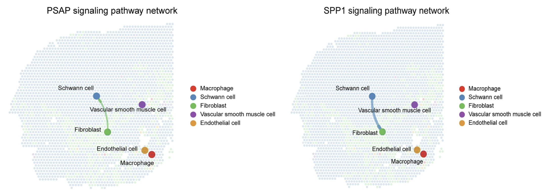
Image source: Dong et al., 2025
Bubble plot
Within CellChat, we can also zoom in on specific ligand-receptor pairs that belong to pathways we have identified. For example, let us take the top 5 pathways and use them as input for netVisual_bubble():
# Top 5 significant pathways
top_pathways <- cellchat_crc@netP$pathways[1:5]
top_pathways[1] "CEACAM" "APP" "COLLAGEN" "MK" "CXCL" In particular, we are interested in the celltypes that are interacting with tumor cells. So we will look at all ligand-receptor complexes in those top pathways that have tumor cells as the target. This is represented as a bubbleplot, where the size of the dot is proportion to the p-value. If a dot does not appear for, this indicates that the interaction is not significant. The color represents the probability of interaction for the celltype-directed interaction, as labeled on the x-axis.
# Number of unique cell types
n_ct <- seurat_rctd@meta.data %>%
pull(first_type) %>%
unique() %>% length()
netVisual_bubble(cellchat_crc,
signaling = top_pathways,
sort.by.source.priority = TRUE,
sources.use = 1:n_ct,
targets.use = "Tumor",
remove.isolate = TRUE,
color.heatmap = "viridis",
angle.x = 90)
In our case, the dots all appear to be the same size. This tells us that the pathways we selected earlier, when a ligand-receptor is significant, it is found to have a very low p-value (very significant).
Zoom in on specific ligand-receptor complexes
Accessing the table of ligand-receptor results
If you wanted to access the full dataframe of results, we can use the subsetCommuncation() function:
df_lr <- subsetCommunication(cellchat_crc) %>%
arrange(desc(prob))
df_lr %>% head(5)| source | target | ligand | receptor | prob | pval | interaction_name | interaction_name_2 | pathway_name | annotation | evidence |
|---|---|---|---|---|---|---|---|---|---|---|
| Tumor | Tumor | CEACAM5 | CEACAM6 | 0.0869136 | 0 | CEACAM5_CEACAM6 | CEACAM5 - CEACAM6 | CEACAM | Cell-Cell Contact | uniprot |
| Tumor | Tumor | CEACAM6 | CEACAM6 | 0.0750469 | 0 | CEACAM6_CEACAM6 | CEACAM6 - CEACAM6 | CEACAM | Cell-Cell Contact | PMID:11590190 |
| T cells | T cells | CXCL12 | CXCR4 | 0.0108678 | 0 | CXCL12_CXCR4 | CXCL12 - CXCR4 | CXCL | Secreted Signaling | KEGG: hsa04060 |
| Tumor | Tumor | MDK | SDC4 | 0.0093137 | 0 | MDK_SDC4 | MDK - SDC4 | MK | Secreted Signaling | PMID: 28356350 |
| Endothelial | Endothelial | PECAM1 | PECAM1 | 0.0087450 | 0 | PECAM1_PECAM1 | PECAM1 - PECAM1 | PECAM1 | Cell-Cell Contact | KEGG: hsa04514 |
From the previous visual, perhaps we were interested in the specific ligand, COL3A1, and receptor, SDC4, interaction between fibroblasts and tumors. We can start by taking a look at the SpatialFeaturePlot() to get a better sense of where these genes localize on our slide:
ligand <- "COL3A1"
receptor <- "SDC4"
SpatialFeaturePlot(crc,
features = c(ligand, receptor),
pt.size.factor = 15,
image.alpha = 0.2)
There is a population of fibroblasts in the tumor cells that appears to correspond with the bins with high COL3A1 expression. Most likely, it is these nearby fibroblasts that are interacting with tumor cells. To confirm that there is higher expression of COL3A1 in fibroblasts, we can use a VlnPlot():
VlnPlot(crc,
features = c(ligand, receptor),
group.by = "first_type",
pt.size = 0,
ncol = 1)
Notably, there is also high expression of SDC4 in the tumor cells. This is the underlying principle of mass action utilized by CellChat. Essentially, if there is high expression of the ligand (COL3A1) in the source celltype (fibroblasts) and high expression of the receptor (SDC4) in the target celltype (tumor cells), then there will be a high probability communication between the two, especially, if they are localized to the same area of the tissue.
Session information
Now that we have completed our analysis, it would be a good time record the packages and versions of the tools we used in the analysis. The sink() function allows us to save the output from a function, in this case the sessionInfo() function. This improves the reproducibility of our code for ourselves and others. We can do this like:
# Create and save a text file with sessionInfo
sink("sessionInfo_spatial_transcriptomics.txt")
sessionInfo()
sink()Reuse
CC-BY-4.0