# Load Visium HD samples and QC
# Visium HD spatial transcriptomics workshop
# Author: Harvard Chan Bioinformatics Core
# Created: May 2026
# Load libraries
library(tidyverse)
library(Seurat)Loading Spatial Data
Spatial transcriptomics
Visium HD
Colorectal Cancer
Learn how to load Visium HD spatial transcriptomics data into R and build Seurat objects. This lesson prepares your spatial dataset for quality control, visualization and downstream analysis.
Keywords
Spatial transcriptomics, Seurat, Tissue slide
Approximate time: 35 minutes
Learning objectives
In this lesson, we will:
- Establish a hypothesis or biological question to assess using the provided dataset
- Quantify how bin size affects the count matrix
- Access important information from a Seurat object
- Create a merged Seurat object from Space Ranger outputs
Overview of lesson
At this point in the experiment, we have sequenced our Visium HD dataset and run it through the Space Ranger pipeline. With the outputs, we will learn what files are necessary to load the data into Seurat. In addition to creating a Seurat object, we will also become familiar with how the Seurat data structure is formatted so that we can access each part of our dataset in future lessons. Once the basics of working in Seurat and R are established, we will then load multiple samples at once in an automated manner.
This is the starting point for a standard spatial transcriptomics analysis!
Exploring the example Visium HD dataset
Throughout this workshop, we will be working with a Visium HD dataset that came from a larger study on human colorectal cancer. The focus of this study was to understand the tumor microenvironment in colorectal cancer (CRC) by utilizing multiple sequencing modalities, including Visium HD, Xenium and FLEX single-cell sequencing.
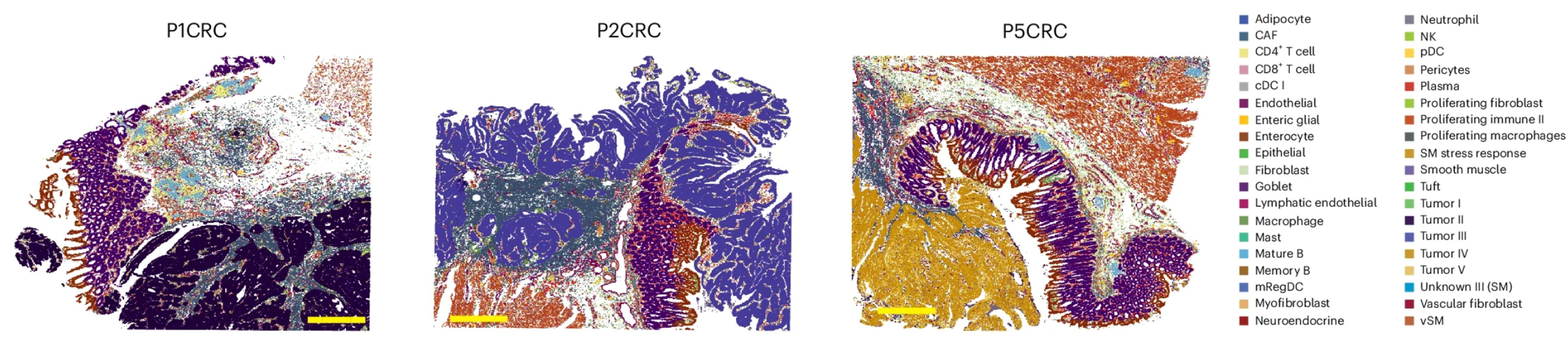
Image source: Oliveira et al. (2025)
In particular, we are going to be working with the P5CRC colorectal cancer sample as there is a matched, normal adjacent P5NAT sample that we can use to compare tumor versus normal tissue.
Dataset availability
This dataset was generated by 10X Genomics and is publicly available on their website here.
Metadata
While it may be tempting to get started right away with loading your data, it is crucial that you first take a moment to document metadata that is associated with your dataset. This information will be important for you to interpret your results correctly as you move further along in your analysis.
For this particular dataset, we have the following metadata available to us about the patient:
- Stage IV-A of CRC
- Female patient
- 58 years old
Additionally, we want to keep track of some basic information that we would expect to see in our dataset, more specifically the cell types we anticipate seeing:
- B cells
- Endothelial cells
- Fibroblasts
- Intestinal epithelial cells
- Myeloid cells
- Neural cells
- Smooth muscle cells
- T cells
- Tumor cells
Sample preparation
It is also good to keep track of the sample preparation and sequencing protocols that were used to generate the data. For this dataset, we know:
- 5 µm sections were taken from the FFPE tissue blocks with a microtome
- Sectioning followed the Visium CytAssist v2 WT Panel Gene Expression protocol
- FFPE tissue sections were placed on plain glass slides for deparaffinization, H&E staining and imaging following the Visium HD FFPE Tissue Preparation Handbook
- Sequencing was performed on an Illumina NovaSeq 6000 with paired-end reads
- Samples were processed with Space Ranger v3.0
- Given the information that we know from the metadata, what might be some questions that we want to answer using our data?
- What are some of the limitations of this dataset that we should keep in mind as we analyze it?
With this information in mind, we can now move forward with loading our data and performing our analysis.
Set up
We have assembled an R Project for you to download that includes the data along with a basic file structure for good data management. Whenever you start a new project, it is a good habit to set up a similar directory structure to clearly organize your data, scripts and results. This will make it easier to keep track of your files and to share your work with others.
Download the data
If you haven’t done this already, the project can be accessed using this link. You will have to left-click the link and select Save Link As... or Download Linked File As..., then select a location on your computer where you would like to place this R Project.
Project organization
When you have large amounts of data (like with spatial transcriptomics), it is easy to lose track of your files and become overwhelmed. We tend to prioritize the analysis and, in the excitement of getting a first look at our data, we often forget to consider how we are going to manage our data and files. This is a common mistake, as data management is often an afterthought when it should be a key part of the workflow from the very beginning. The HMS Data Management Working Group discusses in-depth some aspects to consider beyond the data creation and analysis.
One important aspect of data management is organization. For each experiment you work on and analyze data for, it is considered best practice to get organized by creating a planned storage space. We will do that for our spatial transcriptomics analysis.
Note for Windows OS users
When you open the project folder after unzipping it, please check if you have a spatial_transcriptomics folder with a subfolder also called spatial_transcriptomics. If this is the case, please move all the files from the subfolder into the parent spatial_transcriptomics folder and remove the child spatial_transcriptomics subfolder.
Opening R Studio
We can open the R Project up and see that the provided file structure should look like:
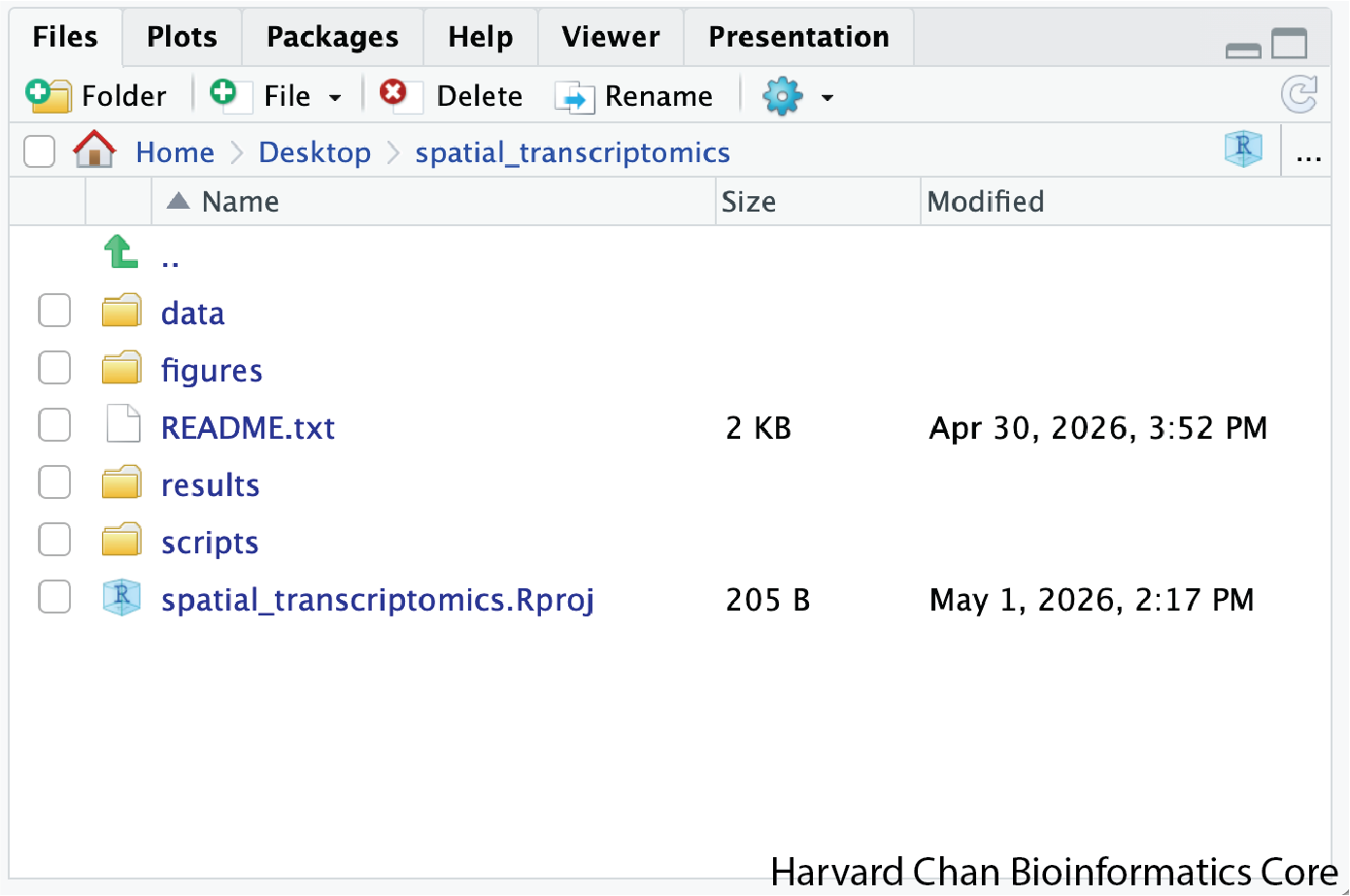
If your R Project looks like above, then you are ready to start!
Cropped images
You may notice that we are working with cropped folders for this workshop. This decision is due to the limitations of how much data can be loaded on a laptop. So here, we have cropped the image so that we have a smaller cross-section of the tissue to work with, ultimately reducing the number of cells for this example dataset.
The code used to create all the files for this workshop can be found here.
New script
Next, open a new Rscript file and start with some comments to indicate what this file is going to contain. Ideally, we will have one script per major step in our analysis. For this first script, we will be loading our data and performing quality control - as indicated in the header.
Loading your libraries at the top of the script will also allow you to easily keep track of which libraries you are using and to load them all at once in the beginning.
Save the Rscript as 01_loading_visium_hd_and_qc.R and place it into the scripts folder. Your working directory should look something like this:
spatial_transcriptomics/
├── data/
│ ├── P5CRC_cropped/
│ ├── P5NAT_cropped/
│ ├── crc_flex_ref_downsample.RDS
│ └── intermediate_seurat/
├── figures/
├── README.txt
├── results/
├── scripts/
│ └── 01_loading_visium_hd_and_qc.R
└── spatial_transcriptomics.RprojLoading data into Seurat
There are several different tools that can be used for loading and analyzing spatial transcriptomics data. While each has their own nuances, they all follow the same fundamental theory and processes:
- Python’s Squidpy
- R’s Spatial Experiment
- R’s Seurat
For this workshop, we will be using the Seurat workflow.
Input files
To load our data, we are going to make use of the function Load10X_Spatial(). The input needed for this function comes from the output generated by Space Ranger, including both the feature matrix and low-resolution tissue image. Once supplied, a Seurat object that contains our counts matrix and image is created.
Using
? to look up function arguments
If you are ever unsure what parameters you can supply to a function, you can make use of the ? call in R. This code will bring up the manual page for the function, which will provide more details on what each variable is used for.
?Load10X_SpatialThere are 3 main arguments that we will be utilizing for this step:
Load10X_Spatial() arguments.
| Argument | Description |
|---|---|
| data.dir | Directory containing the H5 file specified by filename and the image data in a subdirectory called spatial |
| bin.size | Specifies the bin sizes to read in (defaults to c(16, 8)) |
| slice | Name for the stored image of the tissue slice |
Before loading in the data, let us take a look at the files we will be supplying to the function. In particular, let us take a look at sample data/P5CRC_cropped, which is the path we would supply as data.dir in the Load10X_Spatial() function.
data/P5CRC_cropped/
├── binned_outputs
│ ├── square_008um
│ └── square_016um
└── web_summary.htmlIn the Visium HD assay, Space Ranger bins the image into 2µm x 2µm, 8µm x 8µm and 16µm x 16µm bins. The output from each of these resolutions is found in the binned_outputs folder.
How do I know what bin size to use?
This is not an easy question to answer!
The typical recommendation for a Visium HD analysis is to use the 8µm x 8µm resolution of the dataset. However, it is important to consider the dataset you are working with. For example, adipose cells are known to be a larger cell type in size. Therefore, it would be good to consider a large bin size in order to fully represent each cell within a bin. The trade-off for choosing a larger bin size is that the odds of a bin containing multiple cells goes up.
The smaller the bin size is, the more resources it takes to compute anything. So this is the first example (of many) where you must juggle computational practicality and biology when making a decision.
Creating the Seurat object
Now that we understand the input needed for the Load10X_Spatial() function, let’s use it to create a Seurat object called crc. We will specify that we want to load in the 8µm and 16µm bin sizes at the same time.
Typically you would only load in one bin size, but for the purposes of better understanding bins and our Seurat data structure, we will load both here.
crc <- Load10X_Spatial(data.dir = "data/P5CRC_cropped/",
bin.size = c(8, 16),
slice = "P5CRC")We can print out some basic information of our Seurat object to examine its data structure. We will do this frequently throughout the workshop to understand how the Seurat data structure changes with each step of the workflow.
crcAn object of class Seurat
36170 features across 97570 samples within 2 assays
Active assay: Spatial.008um (18085 features, 0 variable features)
1 layer present: counts
1 other assay present: Spatial.016um
2 spatial fields of view present: P5CRC.008um P5CRC.016um
Anatomy of Seurat object
The Seurat object contains many different parts with specific functions to access each slot. To better understand how to access each component, we have created a lesson going through the anatomy of a Seurat object for the crc object we have just created.
We can assess how many bins belong to each bin size by using the ncol() function on our datasets:
ncol(crc[["Spatial.008um"]])[1] 77896ncol(crc[["Spatial.016um"]])[1] 19674- What differences do you see between the
8umand16umbins?
Seurat automatically generates some metadata for each of the cells when the object is created. This information is stored in the @meta.data slot within the Seurat object. The rownames are automatically set to be the cell names.
Note that the 16um columns will contain NA values, which is expected because Seurat will only calculate statistics for the first bin size specified in the bin.size argument.
crc@meta.data %>% View()@meta.data
| orig.ident | nCount_Spatial.008um | nFeature_Spatial.008um | nCount_Spatial.016um | nFeature_Spatial.016um | |
|---|---|---|---|---|---|
| s_008um_00078_00444-1 | s | 65 | 57 | NA | NA |
| s_008um_00128_00278-1 | s | 1300 | 906 | NA | NA |
| s_008um_00052_00559-1 | s | 128 | 121 | NA | NA |
| s_008um_00121_00413-1 | s | 538 | 326 | NA | NA |
| s_008um_00167_00326-1 | s | 44 | 39 | NA | NA |
What does each column represent?
@meta.data
| Column | Description |
|---|---|
| orig.ident | Sample identity if known; defaults to “s” |
| nCount_Spatial | Number of UMIs per cell |
| nFeature_Spatial | Number of genes detected per cell |
While it may seem intimidating at first, the important thing to remember is that this is a dataframe. Therefore, we can modify and work with this dataframe just like we would any other in R!
Loading multiple samples into Seurat
Before we begin, we are going to remove the crc object we have been playing with in order to clear up extra space on our computers. Spatial transcriptomics takes up a lot of memory! So we are being careful to remove any variables that might overload the RAM.
# Delete crc variable to save RAM
rm(crc)Now that we have a better understanding of how to create a Seurat object from Space Ranger outputs, let’s go through how we can load multiple samples at once. In this case we want to represent both samples P5CRC and P5NAT in a singular Seurat object.
Using a for loop
In practice, you will likely have several samples that you will need to read in data for, and that can get tedious and error-prone if you do it one at a time. So, to make the data import into R more efficient, we can use a for loop, which will iterate over a series of commands for each of the inputs given and create Seurat objects for each of our samples.
for loop syntax
We can use for loops in order to iterate over a vector. Each time the loop iterates, it takes an element from the vector and assigns it to a variable, then it processes a series of commands on that variable. Once it has completed all of the commands for that variable, it will take the next element in the vector and repeat the process. This continues until all of the elements in the vector have been processed.
In R, the for loop has the following structure/syntax:
## DO NOT RUN
# For loop syntax
for (element in vector){
command1
command2
command3
}Today, we will use it to iterate over the two sample folders and execute commands for each sample as we did above for a single sample:
Generate path to
data.dirby pasting “_cropped” to the sample nameCreate the Seurat objects from the SpaceRanger data (
Load10X_Spatial())- Set
sliceto sample - Use
bin.sizeof 8um
- Set
Set
orig.identto be sample
Once those steps run, we will store the newly generated Seurat object to a list called list_seurat so that we can eventually merge both samples together.
We will be using a bin size of 8um for the remainder of this workshop!
# List of samples (associated with data.dir)
samples <- c("P5CRC", "P5NAT")
# Empty list to fill with Seurat objects
list_seurat <- list()
for (sample in samples) {
# Path to data directory
data_dir <- paste0("data/", sample, "_cropped")
print(data_dir)
# Create seurat object and set orig ident to be sample
seurat <- Load10X_Spatial(data.dir = data_dir,
bin.size = 8,
slice = sample)
seurat$orig.ident <- sample
# Store seurat object in our list
list_seurat[[sample]] <- seurat
}To confirm that we have succesfully loaded both samples in, we can take a look at the contents of list_seurat. We should see that there are two Seurat objects in our list corresponding to each of our samples.
list_seurat$P5CRC
An object of class Seurat
18085 features across 77896 samples within 1 assay
Active assay: Spatial.008um (18085 features, 0 variable features)
1 layer present: counts
1 spatial field of view present: P5CRC.008um
$P5NAT
An object of class Seurat
18085 features across 91248 samples within 1 assay
Active assay: Spatial.008um (18085 features, 0 variable features)
1 layer present: counts
1 spatial field of view present: P5NAT.008umThis is exactly what we had hoped to see! So now we can move on to the next step, which is merging the samples together into a singular Seurat object.
Merge datasets together
We will merge the samples together because it makes it easier to run the quality control steps. A merged object also enables us to easily compare the data quality for all cells at one time. To create this combined Seurat object, we use the merge() function. Because the same cell IDs can be used in different samples, we add a sample-specific prefix to each of our cell IDs using the add.cell.id argument to ensure the cell names are unique.
# Create singular seurat object out of multiple samples
seurat_merged <- merge(x = list_seurat[["P5CRC"]],
y = list_seurat[["P5NAT"]],
add.cell.id = c("P5CRC", "P5NAT"))
seurat_mergedAn object of class Seurat
18085 features across 169144 samples within 1 assay
Active assay: Spatial.008um (18085 features, 0 variable features)
2 layers present: counts.1, counts.2
2 spatial fields of view present: P5CRC.008um P5NAT.008umFrom the output, we can see that we now have: 2 layers present: counts.1, counts.2
What if I am merging more than two samples?
Seurat has functionality to merge many samples together. You can do this by adding all but one Seurat object to the y argument in a vector format. An example is provided below, assuming you use the list structure we used previously:
## DO NOT RUN
merged_seurat <- merge(x = seurat_list[[1]],
y = seurat_list[2: length(seurat_list)],
add.cell.id = names(seurat_list))The two separate counts indicates that our raw counts matrices are being stored as separate layers in the Seurat object. This is because we have not yet concatenated the matrices together yet with the JoinLayers() function. We want to run this step for two reasons:
- Some calculations may be done on one matrix and not the other
- Later steps will require a singular, joined matrix
# Join layers to get a single counts matrix
seurat_merged <- JoinLayers(seurat_merged)
Merging vs. integration
A common point of confusion is the distinction between integration and merging. In the field, integration is considered to be modifying either your counts or latent space in a way to correct for a batch variable. Whereas what we are doing now is merging or concatenating multiple samples together. This process of merging does not transform the values in the count matrices.
Evaluating merged_seurat
Let’s also double check that we have the correct number of cells. First, let us see what the number of cells was for each sample:
# Sum of cells in P5CRC and P5NAT in seurat_list
ncol(list_seurat[["P5CRC"]]) + ncol(list_seurat[["P5NAT"]])[1] 169144Which is the same as the number of “samples” displayed when we call our Seurat object!
# Check the number of cell/"samples" in merged seurat object
seurat_mergedAn object of class Seurat
18085 features across 169144 samples within 1 assay
Active assay: Spatial.008um (18085 features, 0 variable features)
1 layer present: counts
2 spatial fields of view present: P5CRC.008um P5NAT.008umIf we look at the metadata of the merged Seurat object, we should be able to see the prefixes in the rownames (Cells) as well as the updated orig.ident we set in the for loop earlier.
# Check that the merged object has the appropriate sample-specific prefixes
seurat_merged@meta.data %>% head()@meta.data
| orig.ident | nCount_Spatial.008um | nFeature_Spatial.008um | |
|---|---|---|---|
| P5CRC_s_008um_00078_00444-1 | P5CRC | 65 | 57 |
| P5CRC_s_008um_00128_00278-1 | P5CRC | 1300 | 906 |
| P5CRC_s_008um_00052_00559-1 | P5CRC | 128 | 121 |
| P5CRC_s_008um_00121_00413-1 | P5CRC | 538 | 326 |
| P5CRC_s_008um_00167_00326-1 | P5CRC | 44 | 39 |
seurat_merged@meta.data %>% tail()@meta.data
| orig.ident | nCount_Spatial.008um | nFeature_Spatial.008um | |
|---|---|---|---|
| P5NAT_s_008um_00365_00197-1 | P5NAT | 748 | 488 |
| P5NAT_s_008um_00357_00367-1 | P5NAT | 814 | 454 |
| P5NAT_s_008um_00415_00143-1 | P5NAT | 100 | 25 |
| P5NAT_s_008um_00148_00248-1 | P5NAT | 252 | 222 |
| P5NAT_s_008um_00373_00222-1 | P5NAT | 514 | 436 |
The bin identities are stored as Idents(), which contain the default way to label bins. So the last step here is making sure that the Idents of our bins is a useful piece of information, for example like orig.ident, which contains our sample IDs.
# Set Idents to sample IDs
Idents(seurat_merged) <- "orig.ident"Save!
Now is a great spot to save our seurat_merged object, as the next step is going to be filtering.
# Save integrated Seurat object
saveRDS(seurat_merged, "data/01_seurat_merged.RDS")A good rule of thumb is to save your intermediate objects before any filtration or after running a computationally heavy step that takes a long time to run.
Limited RAM
As we go throughout the workshop, we recommend that you clear your environment after we save an RDS object to avoid taxing your laptop with objects that are too large.
Reuse
CC-BY-4.0