Performing Integration

This lesson guides participants through performing data integration using both canonical correlation analysis (CCA), single cell Variational Inference (scVI), and alternative approaches suitable for more complex integration tasks. Participants will also explore visualization methods such as PCA and UMAP to assess integration quality and gain an introduction to the Harmony algorithm as an alternative strategy for integrating across multiple conditions, batches or protocols.

Keywords

R, Seurat, Scanpy, Integration, CCA, scVI, UMAP, PCA, Harmony

Approximate time: 30 minutes

Learning objectives

In this lesson, we will:

• Perform integration of cells across conditions to identify cells with similar gene expression patterns.
• Describe complex integration tasks and alternative tools for integration.

Overview of lesson

In the last lesson we described in detail the steps of integration. Now, we need to run the code to integrate our data.

Figure 1: Overview of the single-cell RNA-seq workflow.

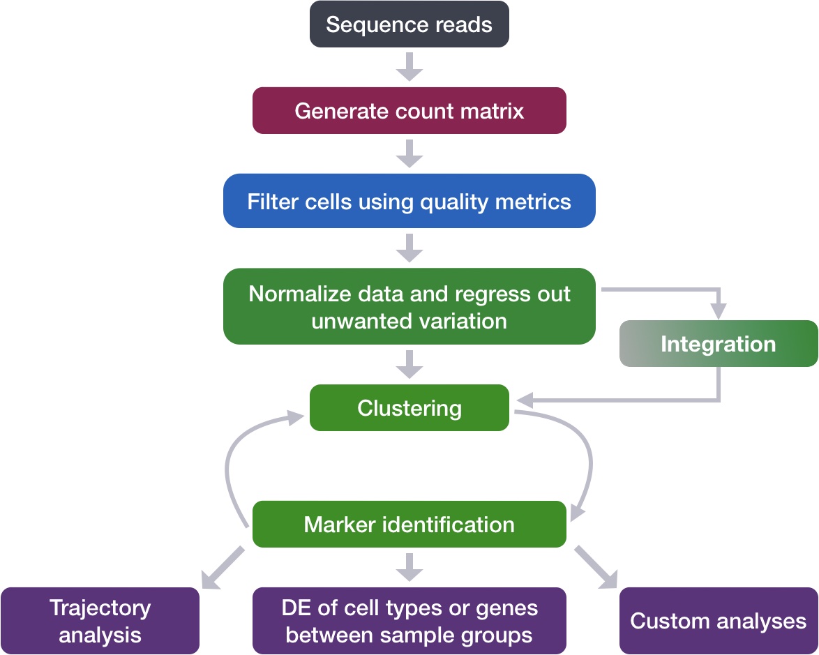
Running integration code

The R, Seurat workflow uses CCA while the Python, scanpy workflow uses scVI.

R

We will start by using our SCTransform object as input, let’s perform the integration across conditions (ctrl and stim).

Loading split_seurat

If you are missing the split_seurat object in your environment, you can first load it from your data folder:

# Load the split seurat object into the environment
split_seurat <- readRDS("intermediate/07_split_seurat.RDS")

If you do not have the split_seurat.rds file in your data folder, you can right-click here to download it to the data folder (it may take a bit of time to download).

TODO: double check this link

Let’s recall where we left off. We created a new object called split_seurat which is a named list containing two seurat object - corresponding with our two samples. After splitting the dataset, we applied the SCTransform normalization to each sample individually.

split_seurat

$ctrl
An object of class Seurat 
27864 features across 14847 samples within 2 assays 
Active assay: SCT (13799 features, 3000 variable features)
 3 layers present: counts, data, scale.data
 1 other assay present: RNA
 1 dimensional reduction calculated: pca

$stim
An object of class Seurat 
27760 features across 14782 samples within 2 assays 
Active assay: SCT (13695 features, 3000 variable features)
 3 layers present: counts, data, scale.data
 1 other assay present: RNA
 1 dimensional reduction calculated: pca

Now, we need to identify the shared variable genes for the integration. By default, this function only selects the top 2,000 genes. In this step Seurat performs a more complex version of an intersect between the highly variable genes from each condition (based on SCTransform). We have specified 3,000 genes for the size of the intersect set.

# Select the most variable features to use for integration
integ_features <- SelectIntegrationFeatures(object.list = split_seurat,
                                            nfeatures = 3000)

Now, we need to prepare the SCTransform object for integration. This function basically prepares for integration analysis by ensuring all necessary data (specifically the SCTransform residuals) are present for the features chosen as anchors between datasets.

# Prepare the SCT list object for integration
split_seurat <- PrepSCTIntegration(object.list = split_seurat, 
                                   anchor.features = integ_features)

Now, we are going to perform CCA, find the best buddies or anchors and filter incorrect anchors. For our dataset, this will take up to 15 minutes to run. Also, note that the progress bar in your console will stay at 0%, but know that it is actually running.

# Find best buddies - can take a while to run
integ_anchors <- FindIntegrationAnchors(object.list = split_seurat, 
                                        normalization.method = "SCT", 
                                        anchor.features = integ_features)

Finally, we can integrate across conditions.

# Integrate across conditions
seurat_integrated <- IntegrateData(anchorset = integ_anchors, 
                                   normalization.method = "SCT")

In the process of splitting our seurat object, we also split the counts matrices in our RNA assay. So we will run the JoinLayers() function to ensure that all our matrices are combined correctly.

# Rejoin the layers in the RNA assay that we split earlier
seurat_integrated[["RNA"]] <- JoinLayers(seurat_integrated[["RNA"]])

Python

To run scVI, we first need to specify what our batch_key (sample) and categorical_covariate_keys (unwanted variation) are. This information gets stored in the AnnData object with the scvi.model.SCVI.setup_anndata() function. Then, we initialize the model (variational autoencoder architecture) so that we can run the next step, which is training the model.

We can see the basic information about the model by printing out the model variable created:

# Create new anndata for integration
adata_integrated = adata_phase.copy()

# Set parameters for the scVI model
scvi.model.SCVI.setup_anndata(adata_integrated, 
                              layer = "counts", 
                              batch_key = "sample", 
                              categorical_covariate_keys =[ "phase", "mitoFr"])

model = scvi.model.SCVI(adata_integrated, 
                        n_layers = 2, 
                        n_latent = 30, 
                        gene_likelihood = "nb")
model

SCVI model with the following parameters: 
n_hidden: 128, n_latent: 30, n_layers: 2, dropout_rate: 0.1, dispersion: gene, 
gene_likelihood: nb, latent_distribution: normal.
Training status: Not Trained
Model's adata is minified?: False

scVI uses the concept of variational autoencoders to build neural networks (encoder and decoder) that are capable of reconstructing the original count information. To accomplish this goal, several back‑and‑forth iterations between the two networks are necessary in order to ensure the accuracy of the reconstruction.

Epochs

The number of epochs specifies how many iterations of the model training will be done. The more epochs will improve the results of the training. Here we have set it to 100 to reduce the amount of time this step takes to run while retaining the accuracy of the results.

By default the number of epochs is typically greater than 200.

# Train encoder and decoder neural networks
# This step will take several minutes
model.train(max_epochs = 100)

We use the get_latent_representation() function to generate a new latent space (like PCA) that reduces the dimensionality of our dataset while taking into consideration the batch variable we specified earlier. This new latent space, which we store as X_scvi can later be used to calculate our nearest neighbors and UMAP coordinates.

# Store resultant latent space
adata_integrated.obsm["X_scvi"] = model.get_latent_representation()

We now have our new scVI values stores in our adata_integrated object within the obsm slot, just like we had when we ran PCA.

# Note the new scVI value stored in the obsm slot
adata_integrated

AnnData object with n_obs × n_vars = 29629 × 14167
    obs: 'n_genes', 'sample', 'n_genes_by_counts', 'total_counts', 'cells', 'log10GenesPerUMI', 'log1p_n_genes_by_counts', 'log1p_total_counts', 'pct_counts_in_top_50_genes', 'pct_counts_in_top_100_genes', 'pct_counts_in_top_200_genes', 'pct_counts_in_top_500_genes', 'total_counts_mito', 'log1p_total_counts_mito', 'pct_counts_mito', 'mito_ratio', 'S_score', 'G2M_score', 'phase', 'mitoFr', '_scvi_batch', '_scvi_labels'
    var: 'gene_ids', 'feature_types', 'n_cells_by_counts', 'mean_counts', 'pct_dropout_by_counts', 'total_counts', 'mito', 'log1p_mean_counts', 'log1p_total_counts', 'n_counts', 'highly_variable', 'highly_variable_rank', 'means', 'variances', 'variances_norm', 'highly_variable_nbatches'
    uns: '_scvi_manager_uuid', '_scvi_uuid', 'hvg', 'log1p', 'pca', 'phase_colors', 'sample_colors'
    obsm: 'X_pca', 'X_scvi', '_scvi_extra_categorical_covs'
    varm: 'PCs'
    layers: 'counts', 'log', 'median', None (.X)

Dimensionality reduction assessment

After integration, to visualize the integrated data we can use dimensionality reduction techniques, such as PCA and Uniform Manifold Approximation and Projection (UMAP). We are hoping to see that cells from each batch overlay nicely in the reduced dimensions.

R

With CCA, we have created a new integrated assay with our modified expression matrix. Therefore, we need to once again run our PCA calculation using these updates values.

# Run PCA
seurat_integrated <- RunPCA(object = seurat_integrated)

Using the seurat_phase object, we can directly compare the before and after integration PCA representation.

# Plot unintegrated PCA
p_unint <- PCAPlot(seurat_phase,
                   group.by = "sample")

# Plot integrated PCA
p_int <- PCAPlot(seurat_integrated,
                 group.by = "sample")

p_unint + p_int

Figure 2: Contrast the latent representation after CCA integration vs. unintegrated PCA.

Python

Now we can compare and contrast the latent representation that was calculated with PCA and the new SCVI representation. This allows us to see what batch correction has been accomplished.

# Create plot with the correct dimensions
fig, axes = plt.subplots(1, 2, figsize=(10, 5))

# Plot unintegrated PCA
sc.pl.embedding(adata_integrated, basis='X_pca', 
                color='sample', ax=axes[0], 
                title="PCA", show=False)
# Plot integrated scVI latent space
sc.pl.embedding(adata_integrated, basis='X_scvi', 
                color='sample', ax=axes[1], 
                title="SCVI", show=False)

plt.tight_layout()
plt.show()

Figure 3: Contrast the latent representation after scVI integration vs. unintegrated PCA.

We now have good overlapping of each batch in our dataset! However, this visual representation is a bit subjective, so we will use several different ways to confirm whether or not the integration was successful in future lessons.

Save integrated object

Since integration requires a lot of compute resources and can take a lot of time to run, it is a good idea to save the integrated object so that you do not have to re-run this step many times.

R

# Save integrated Seurat object
saveRDS(seurat_integrated, "data/integrated_seurat.rds")

Python

# Save integrated adata object
adata_integrated.write_h5ad("data/adata_integrated.h5ad")

Complex Integration Tasks

It is important to recognize that alternative integration algorithms exist and may work better for more complex integration tasks (see Luecken et al. (2022) for a comprehensive review).

Not all integration algorithms rely on the same methodology, and they do not always provide the same type of corrected output (embeddings, count matrix…). Their performance is also affected by preliminary data processing steps, including which normalization method was used and how highly variable genes (HVGs) were determined. All those considerations are important to keep in mind when selecting a data integration approach for your study.

What do we mean by a “complex” integration task?

In their benchmarking study, Luecken et al. (2022) compared the performance of different scRNA-seq integration tools when confronted to different “complex” tasks. The “complexity” of integrating a dataset may relate to the number of samples (perhaps generated using different protocols) but also to the biological question the study seeks to address (e.g. comparing cell types across tissues, species…). In these contexts, you may need to integrate across multiple confounding factors before you can start exploring the biology of your system.

Figure 4: Examples of complex single-cell integration scenarios across donors, technologies, tissues, and conditions.

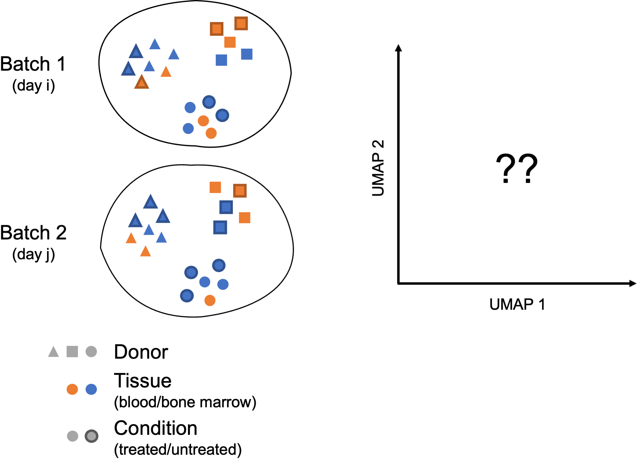
In these more complex scenarios, you want to select a data integration approach that successfully balances out the challenges of batch correction while preserving meaningful biological variation.

Not all tools may perform as well on every task, and complex datasets may require testing several data integration approaches. You might want to analyze independently each of the batches you consider to integrate across, in order to define cell identities at this level before integrating and checking that the initially annotated cell types are mixed as expected.

Harmony integration

Harmony was developed in 2019 and is an example of a tool that can handle complex integration tasks. From benchmarking studies, it has been shown to perform well for single-cell datasets at integrating datasets with strong batch effects.

Harmony applies a series of iterative corrections to our PCA space.

Figure 5: Overview of the Harmony algorithm for batch correction and integration of single-cell datasets.
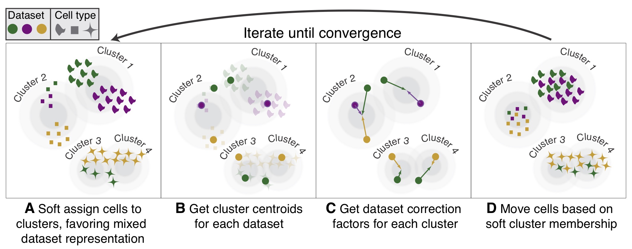
Image Source: Korsunsky et al. (2019)

The following steps are taken:

1. k-means clustering to identify clusters in PCA space.
2. Calculate a “diversity” score for each cluster, reflecting if it contains a balanced amounts of cells from each of the batches (donor, condition, tissue, technology, etc.)
3. Harmony determines how much a cell’s batch identity impacts its PC coordinates and applies a correction to “shift” the cell towards the centroid of the cluster it belongs to.
4. Cells are projected again using these corrected PCs and the process is repeated iteratively until convergence.

Harmony notably presents the following advantages (Korsunsky et al. 2019, Tran et al. (2020)):

• Possibility to integrate data across several variables (for example, by experimental batch and by condition)
• Significant gain in speed and lower memory requirements for integration of large datasets
• Interoperability with the Seurat workflow

Harmony is available within the Seurat workflow with the RunHarmony() function, but is also a stand-alone package. For a more detailed breakdown of the Harmony algorithm, we recommend checking this advanced vignette from the package developers.

Implementing Harmony within the Seurat workflow

In practice, we can easily use Harmony within our Seurat workflow. To perform integration, Harmony takes as input a merged Seurat object, containing data that has been appropriately normalized (i.e. here, normalized using SCTransform) and for which highly variable features and PCs are defined.

There are 2 ways to create the input:

1. Merge the raw Seurat objects for all samples to integrate; then perform normalization, variable feature selection and PC calculation on this merged object (workflow recommended by Harmony developers)
2. Perform (SCT) normalization independently on each sample and find integration features across samples using Seurat; then merge these normalized Seurat objects, set variable features manually to integration features, and finally calculate PCs on this merged object (workflow best reflecting recommendations for application of SCTransform)

In the first scenario, assuming raw_seurat_list is a list of N samples containing raw data that have only undergone QC filtering, we would thus run the following code:

# Merge raw samples
merged_seurat <- merge(x = raw_seurat_list[[1]],
               y = raw_seurat_list[2:length(raw_seurat_list)],
               merge.data = TRUE)

# Perform log-normalization and feature selection, as well as SCT normalization on global object
merged_seurat <- merged_seurat %>%
    NormalizeData() %>%
    FindVariableFeatures(selection.method = "vst", nfeatures = 2000) %>% 
    ScaleData() %>%
    SCTransform(vars.to.regress = c("mitoRatio"))

# Calculate PCs using variable features determined by SCTransform (3000 by default)
merged_seurat <- RunPCA(merged_seurat, assay = "SCT", npcs = 50)

In the second scenario, assuming norm_seurat_list is a list of N samples similar to our split_seurat object, i.e. containing data that have been normalized as demonstrated in the previous lecture on SCT normalization, we would thus run the following code:

# Find most variable features across samples to integrate
integ_features <- SelectIntegrationFeatures(object.list = norm_seurat_list, nfeatures = 3000)

# Merge normalized samples
merged_seurat <- merge(x = norm_seurat_list[[1]],
               y = norm_seurat_list[2:length(raw_seurat_list)],
               merge.data = TRUE)
DefaultAssay(merged_seurat) <- "SCT"

# Manually set variable features of merged Seurat object
VariableFeatures(merged_seurat) <- integ_features

# Calculate PCs using manually set variable features
merged_seurat <- RunPCA(merged_seurat, assay = "SCT", npcs = 50)

Make an educated choice on which integration method to use

As mentioned above, there is active discussion within the community regarding which of those 2 approaches to use (see for example here and here). We recommend that you check GitHub forums to make your own opinion and for updates.

Regardless of the approach, we now have a merged Seurat object containing normalized data for all the samples we need to integrate, as well as defined variable features and PCs.

One last thing we need to do before running Harmony is to make sure that the metadata of our Seurat object contains one (or several) variable(s) describing the factor(s) we want to integrate on (e.g. one variable for sample_id, one variable for experiment_date).

We’re then ready to run Harmony!

harmonized_seurat <- RunHarmony(merged_seurat, 
                group.by.vars = c("sample_id", "experiment_date"), 
                reduction = "pca", assay.use = "SCT", reduction.save = "harmony")

Many covariates

You can specify however many variables to integrate on using the group.by.vars parameter, although we would recommend keeping these to the minimum necessary for your study.

The line of code above adds a new reduction of 50 “harmony components” (~ corrected PCs) to our Seurat object, stored in harmonized_seurat@reductions$harmony

To make sure our Harmony integration is reflected in the data visualization, we still need to generate a UMAP derived from these harmony embeddings instead of PCs:

harmonized_seurat <- RunUMAP(harmonized_seurat, reduction = "harmony", assay = "SCT", dims = 1:40)

Finally, when running the clustering analysis later on (see next lecture for details), we will also need to set the reduction to use as “harmony” (instead of “pca” by default).

harmonized_seurat <- FindNeighbors(object = harmonized_seurat, reduction = "harmony")
harmonized_seurat <- FindClusters(harmonized_seurat, resolution = c(0.2, 0.4, 0.6, 0.8, 1.0, 1.2))

The rest of the Seurat and scanpy workflow and downstream analyses after integration using Harmony can then proceed without further amendments.

---

Next Lesson >>

Back to Schedule