Loading Single-cell RNA-seq Data

In this lesson, participants learn how to load single‑cell RNA‑seq count data. The lesson introduces the structure of typical 10X Genomics output files and how to import these files for multiple samples into R/Python. Participants explore the structure of the single-cell object. By the end, participants will be able to prepare their data for downstream quality control and analysis.

Keywords

data import, 10X Genomics, Seurat, scanpy

Approximate time: 90 minutes

Learning objectives

In this lesson, we will:

• Set-up the environment for a single-cell analysis.
• Establish good data management and metadata practices.
• Demonstrate how to import data and set up a project for upcoming quality control analysis.

Overview of lesson

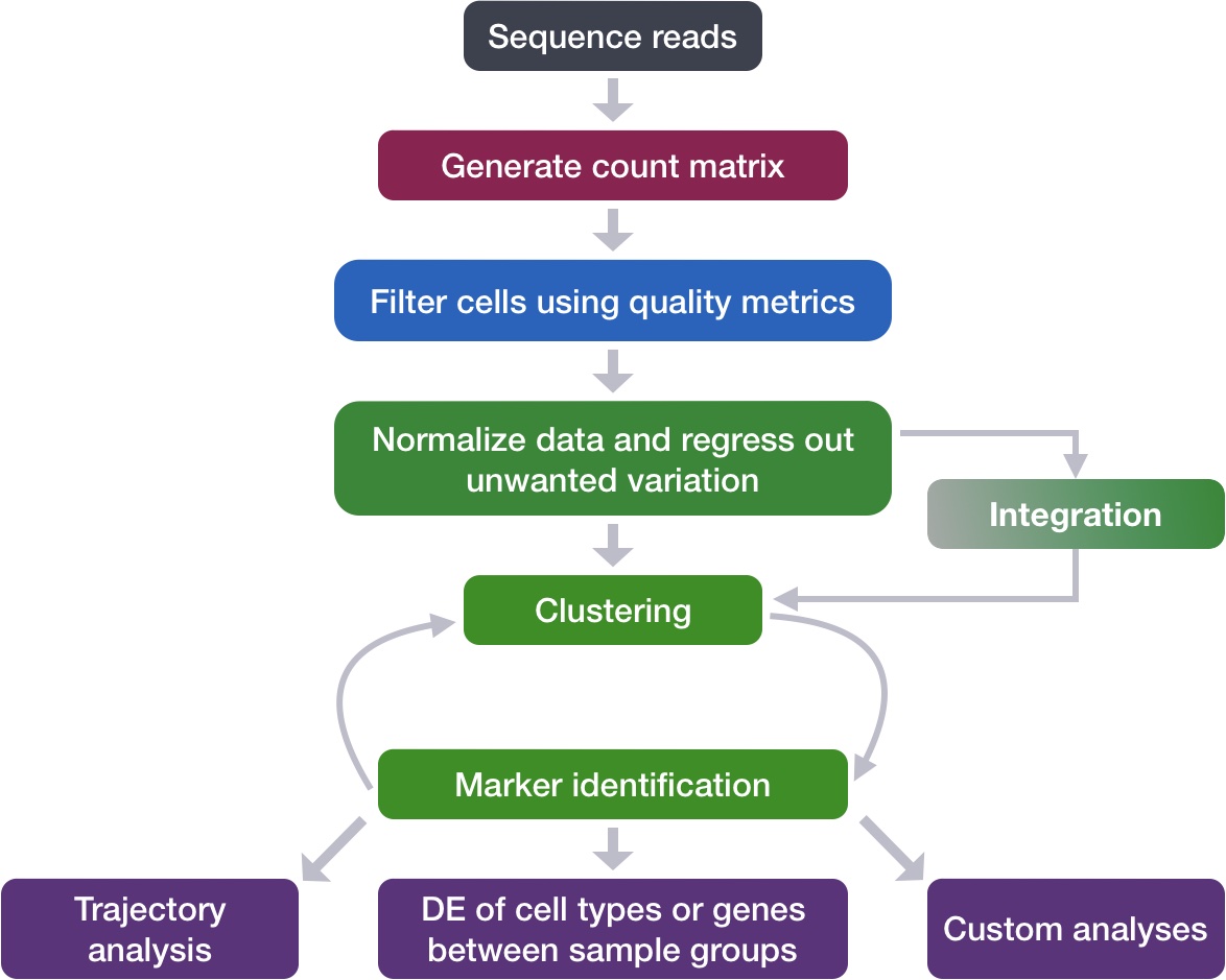
To begin a standard single-cell analysis, we must first understand the dataset we are working with. Then, assuming the data has already been generated, we must load the gene expression counts into our programming language of choice (R or Python). This will enable us to move on to the next step of the workflow, which is assessing the quality of the data to filter cells using quality metrics.

Figure 1: Overview of the single-cell RNA-seq workflow.

Exploring the example dataset

For this workshop, we will be working with a single-cell RNA-seq dataset which is part of a larger study from Kang et al. (2017). In this paper, the authors present a computational algorithm that harnesses genetic variation (eQTL) to determine the genetic identity of each droplet containing a single cell (singlet) and identify droplets containing two cells from different individuals (doublets).

The data used to test their algorithm consists of pooled Peripheral Blood Mononuclear Cells (PBMCs) taken from eight lupus patients, split into control and interferon beta-treated (stimulated) conditions.

Figure 2: Overview of the Kang et al. (2017) pooled PBMC single-cell RNA-seq study design.
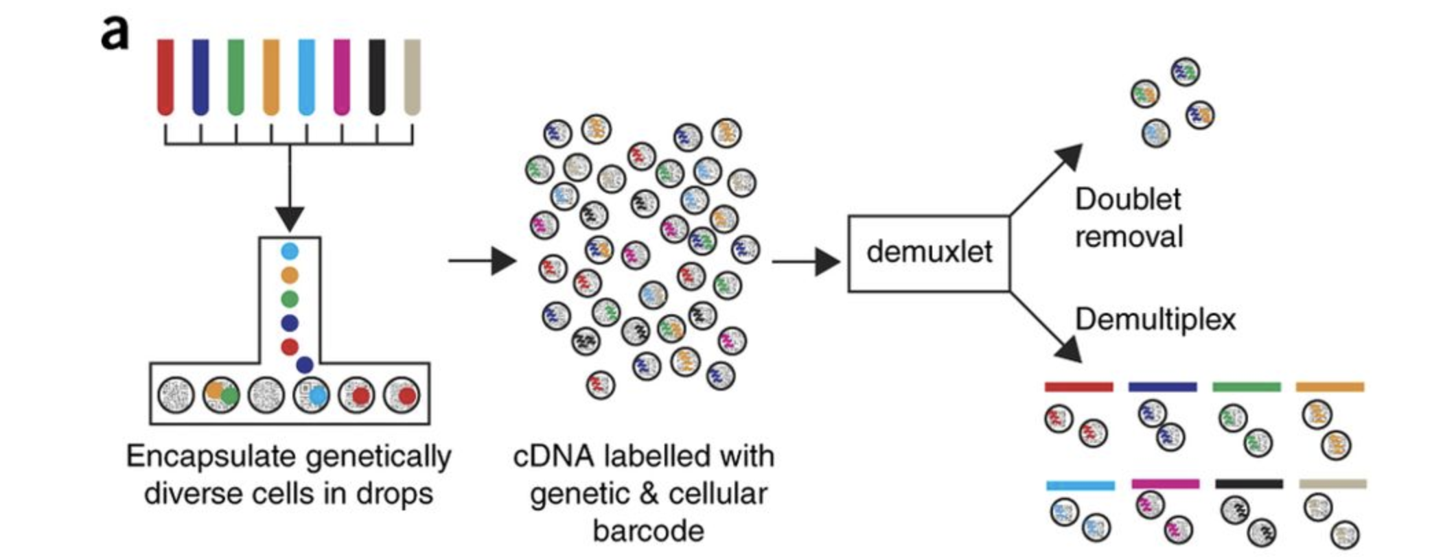
Image credit: Kang et al. (2017)

Downloading the raw data

This dataset is available on GEO (GSE96583), however the available counts matrix lacked mitochondrial reads, so we downloaded the BAM files from the SRA (SRP102802). These BAM files were converted back to FASTQ files, then run through Cell Ranger to obtain the count data that we will be using.

The count data for this dataset is also freely available from 10X Genomics and in several popular tutorials, including the Seurat PBMC tutorial.

Metadata

In addition to the raw data, we also need to collect information about the data; this is known as metadata. There is often a temptation to just start exploring the data, but it is not very meaningful if we know nothing about the samples the data originated from.

Some relevant experimental metadata for our dataset is provided below:

• PBMC samples from eight individual lupus patients were separated into two aliquots each.
• One aliquot of PBMCs was activated by 100 U/mL of recombinant IFN-β for 6 hours and the second aliquot was left untreated.
• After 6 hours, the eight samples for each condition were pooled together in two final pools (stimulated cells and control cells). We will be working with these two, pooled samples.
• The libraries were prepared using 10X Genomics version 2 chemistry and sequenced on the Illumina NextSeq 500.
• 12,138 and 12,167 cells were identified (after removing doublets) for control and stimulated pooled samples, respectively.

Pooling samples together

We did not demultiplex the samples because SNP genotype information was used to demultiplex in the paper and the barcodes/sample IDs were not readily available for this data. Generally, you would demultiplex and perform QC on each individual sample rather than pooling the samples.

Therefore we are unable to identify which of the eight individuals a cell comes from for this example analysis.

It is recommended that you have some expectation regarding the cell types you expect to see in a dataset prior to performing the QC. This will inform you if you have any cell types with low complexity (lots of transcripts from a few genes) or cells with higher levels of mitochondrial expression. This will enable us to account for these biological factors during the analysis workflow.

Since the samples are PBMCs, we will expect immune cells, such as:

• B cells
• T cells
• NK cells
• Monocytes
• Macrophages
• Possibly megakaryocytes

None of the above cell types are expected to be low complexity or anticipated to have high mitochondrial content.

Exercise 1

1. Given the information that we know from the metadata, what might be some questions that we want to answer using our data?
2. What are some of the limitations of this dataset that we should keep in mind as we analyze it?

Set up

For this workshop, we will be working with the files and folders that have been pre-generated for you.

Download data

If you haven’t done this already, the project can be accessed using this link.

Once downloaded, you should see a file called scrna_python_r_update.zip on your computer (likely, in your Downloads folder).

1. Unzip this file. It will result in a folder of the same name.
2. Move the folder to the location on your computer where you would like to perform the analysis. We typically recommend putting it in the Desktop folder.
3. Unzip the scrna_python_r_update folder and open it.

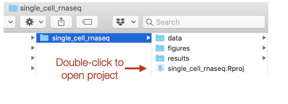
Figure 3: Project directory structure for the single_cell_rnaseq workshop materials.

The data/ folder is already populated with the input files that will be used throughout the workshop.

Note for Windows OS users

When you open the project folder after unzipping, please check if you have a data folder with a subfolder also called data. If this is the case, please move all the files from the subfolder into the parent data folder.

Project organization

One of the most important parts of research that involves large amounts of data is how best to manage it. We tend to prioritize the analysis, but there are many other important aspects of data management that are often overlooked in the excitement to get a first look at new data. The HMS Data Management Working Group, discusses in-depth some things to consider beyond the data creation and analysis.

One important aspect of data management is organization. For each experiment you work on and analyze data for, it is considered best practice to get organized by creating a planned storage space (directory structure). We will do that for our single-cell analysis.

Look inside your project space and you will find that a directory structure has been set-up for you:

scrna_python_r_update/
├── data
├── figures
└── results

New script and loading libraries

R

Locate the .Rproj file and double-click on it. This will open up RStudio with the “single_cell_rnaseq” project loaded. Next, open a new Rscript file, and start with some comments to indicate what this file is going to contain:

# Load 10x single-cell data
# Introduction to single-cell RNA-seq workshop
# Author: Harvard Chan Bioinformatics Core
# June 2026

Save the Rscript as quality_control.R. Your working directory should look something like this:

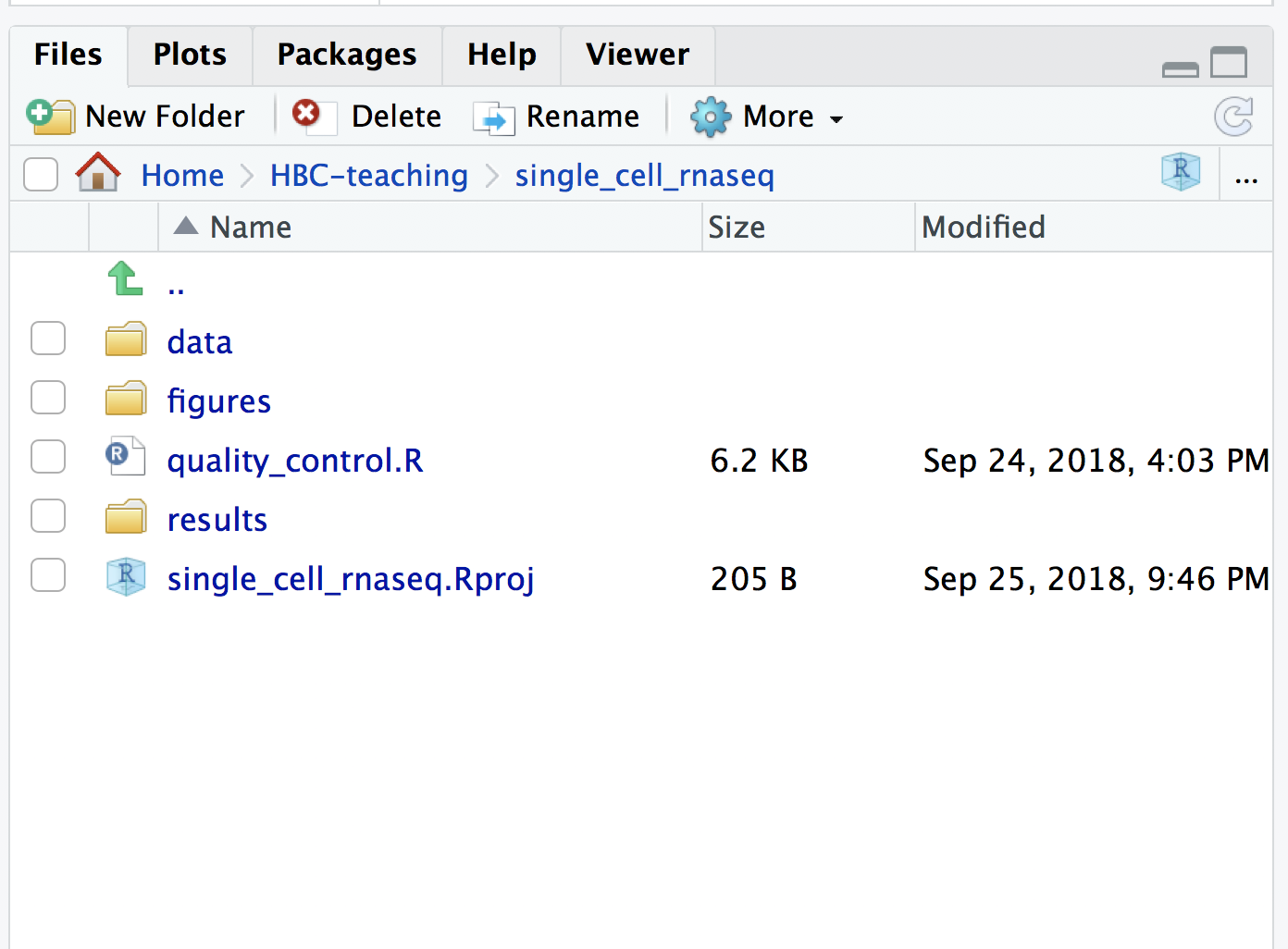
Figure 4: RStudio interface with the single_cell_rnaseq project opened.

Now, we can load the necessary libraries:

# Load libraries
library(Seurat)
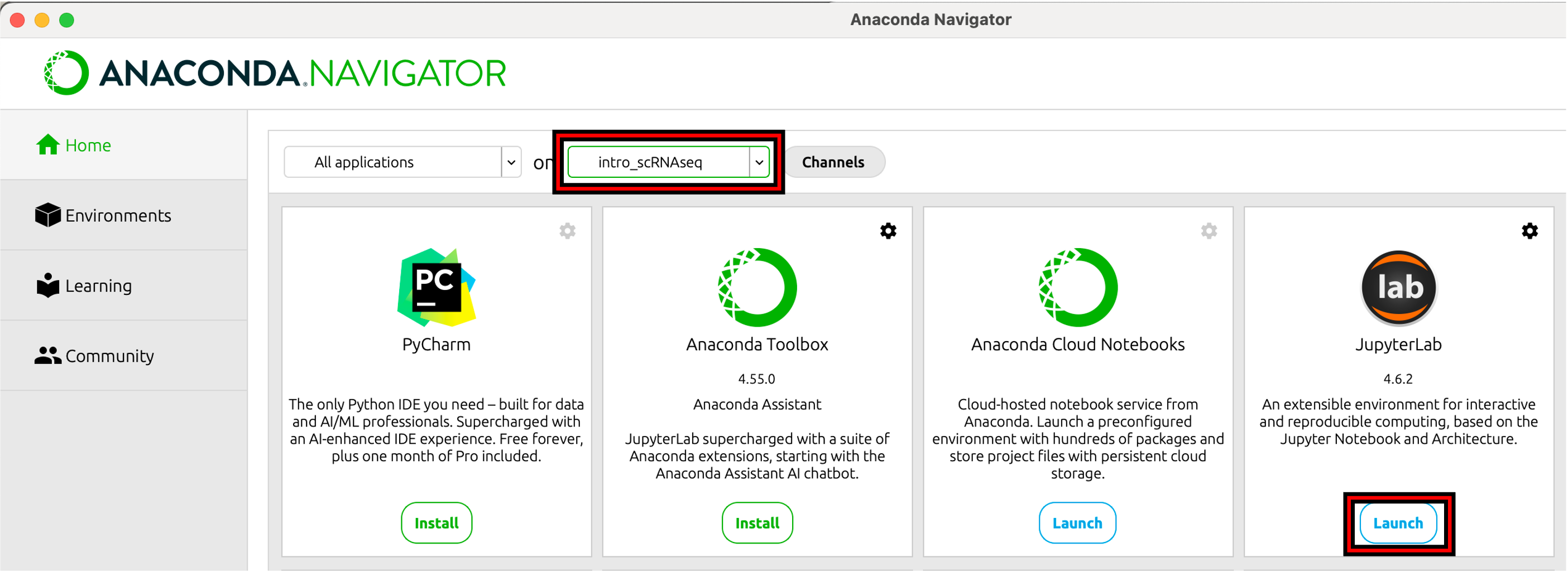
library(tidyverse)

Python

Open Anaconda Navigator and set the environment to the intro_scRNAseq environment that we installed all our packages into. Then hit the “Launch” button under Jupyter Lab to open the notebook interface.

Figure 5: Anaconda Navigator, with conda environment and launch button for Jupyter Lab highlighted.

In the File Explorer of Jupyter Lab, navigate to where you downloaded and unzipped the files in the previous step. In the screenshot here, you can see that we navigated to “Desktop” -> “scrna_python_r_update”:

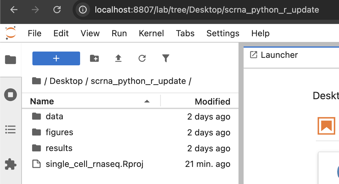
Figure 6: File explorer with Jupyter Lab, navigating to where the downloaded scrna_python_r_update folder is stored.

The single_cell_rnaseq.Rproj file

For the Python version of this workshop, we will ignore the single_cell_rnaseq.Rproj file. This is meant to be used with the R based workflow and is not applicable for the python instructions.

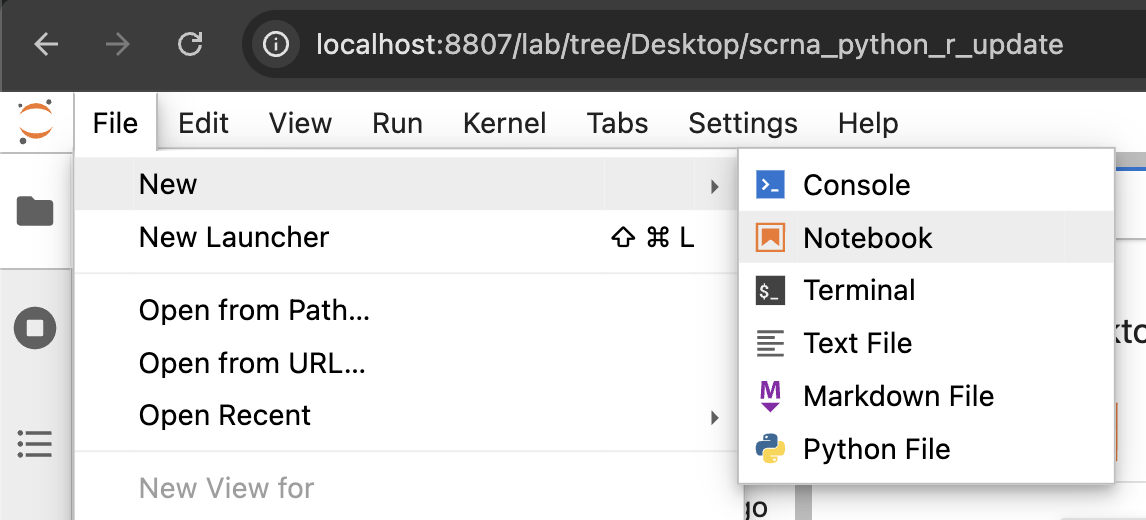
Now that we are in the correct project directory, we can create a new Jupyter Lab notebook to begin programming.

Figure 7: Create a new “Notebook” from the “File” tab of Jupyter Lab.

A pop-up will appear to Select Kernel. We are going to select the intro_scRNA kernel in order to use all the packages we installed previously.

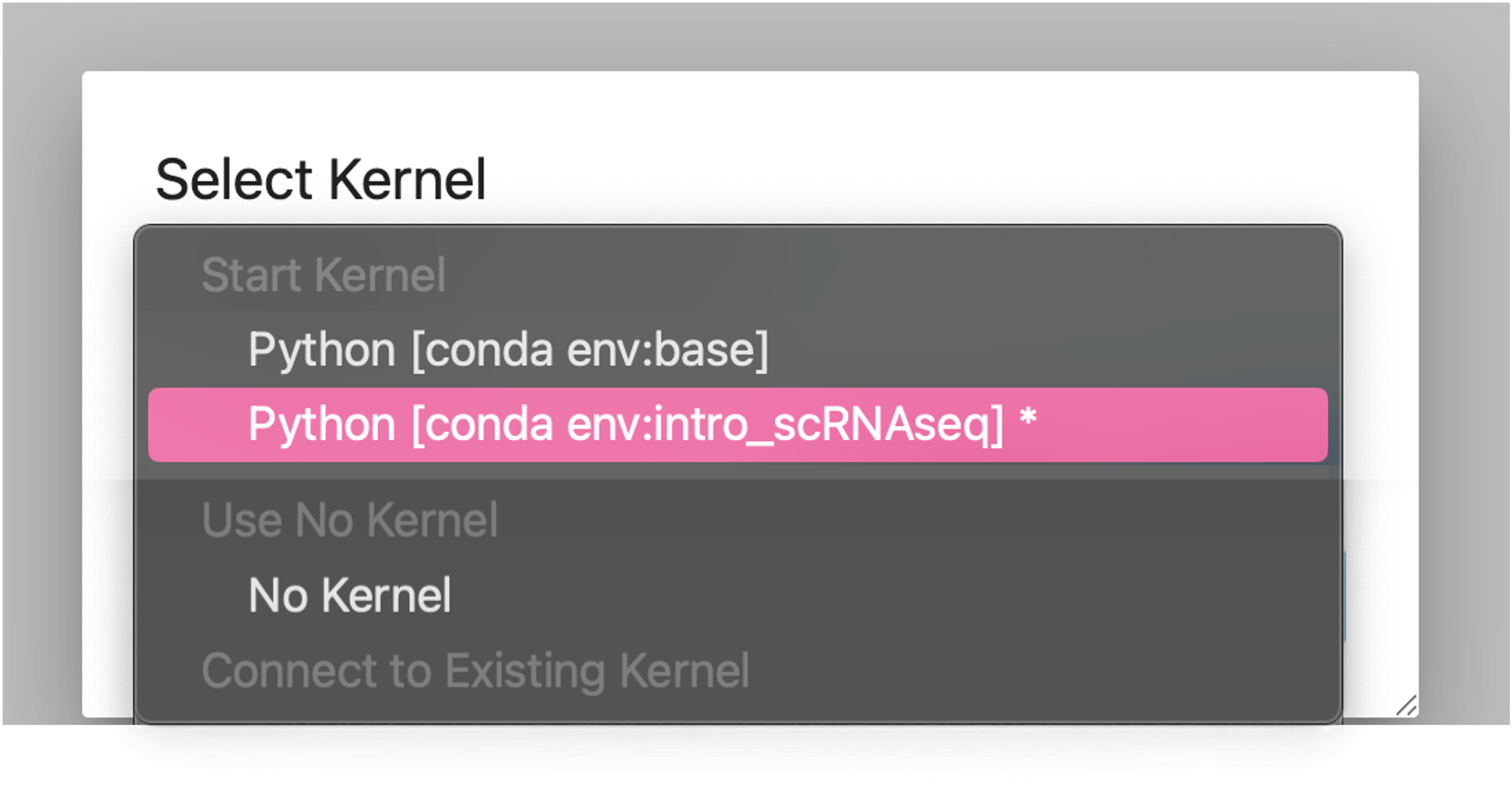
Figure 8: Select the intro_scRNA kernel for the Jupyter Notebook.

Rename the notebook to be quality_control.ipynb.

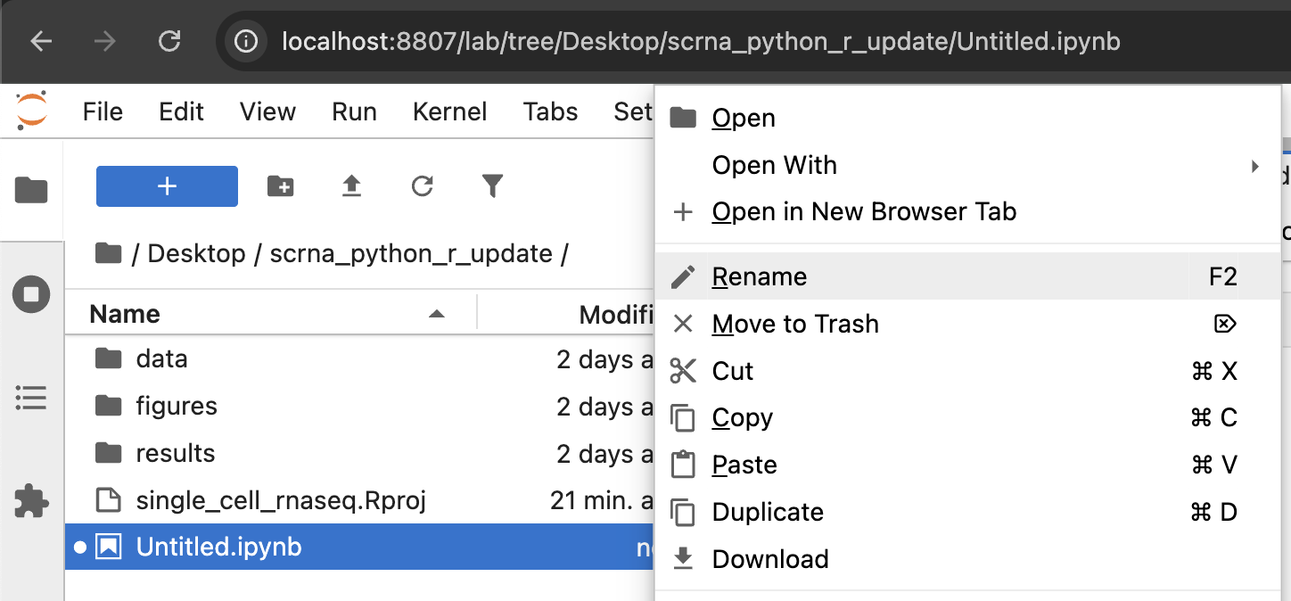
Figure 9: Rename the new Untitled.ipynb file to quality_control.ipynb.

In the first cell, we are going to add some comments to indicate what this file is going to contain:

# Load 10x single-cell data
# Introduction to single-cell RNA-seq workshop
# Author: Harvard Chan Bioinformatics Core
# June 2026

Next, we can import the necessary packages:

# Load packages
import scanpy as sc
import numpy as np
import seaborn as sns
import anndata
import matplotlib.pyplot as plt

Which should give a Jupyter Notebook that looks like this:

Figure 10: Final set-up of Jupyter Notebook for the scRNA-seq workshop.

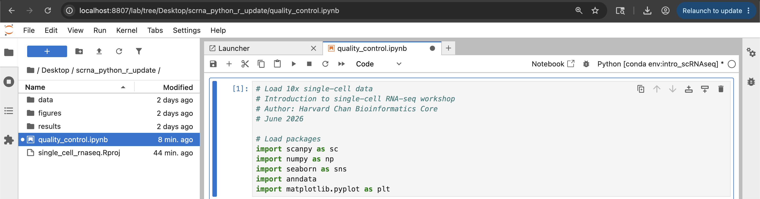
Data files used as input

After processing 10X data using its proprietary software Cell Ranger, you will have an outs directory (always). Within this directory you will find a number of different files including the files listed below:

File / Folder	Description
web_summary.html	Report that explores different QC metrics, including the mapping metrics, filtering thresholds, estimated number of cells after filtering, and information on the number of reads and genes per cell after filtering.
BAM alignment files	Files used for visualization of the mapped reads and for re-creation of FASTQ files, if needed
filtered_feature_bc_matrix	Folder containing all files needed to construct the count matrix using data filtered by Cell Ranger
raw_feature_bc_matrix	Folder containing all files needed to construct the count matrix using the raw unfiltered data

While Cell Ranger performs filtering on the expression counts (see note below), we wish to perform our own QC and filtering because we want to account for the biology of our experiment/biological system. Given this, we are only interested in the raw_feature_bc_matrix folder in the Cell Ranger output.

Why don’t we use the filtered_feature_bc_matrix folder?

The filtered_feature_bc_matrix uses internal filtering criteria by Cell Ranger, and we do not have control of what cells to keep or abandon.

The filtering performed by Cell Ranger when generating the filtered_feature_bc_matrix is often good; however, sometimes data can be of very high quality and the Cell Ranger filtering process can remove high quality cells.

In addition, it is generally preferable to explore your own data while taking into account the biology of the experiment for applying thresholds during filtering. For example, if you expect a particular cell type in your dataset to be smaller and/or not as transcriptionally active as other cell types in your dataset, these cells have the potential to be filtered out. However, with Cell Ranger v3 they have tried to account for cells of different sizes (for example, tumor vs infiltrating lymphocytes), and now may not filter as many low quality cells as needed.

Regardless of the technology or pipeline used to process your raw single-cell RNA-seq sequence data, the output with quantified expression will generally be the same. That is, for each individual sample you will have the following three files:

1. A file with the cell IDs, representing all cells quantified
2. A file with the gene IDs, representing all genes quantified
3. A matrix of counts per gene for every cell

We can explore these files by clicking the data/ctrl_raw_feature_bc_matrix folder:

barcodes.tsv

This is a text file which contains all cellular barcodes present for that sample. Barcodes are listed in the order of data presented in the matrix file (i.e. these are the column names).

Table 1: First several rows of the barcodes.tsv.gz file

X1
AAACATACAAAACG-1
AAACATACAAAAGC-1
AAACATACAAACAG-1
AAACATACAAACGA-1
AAACATACAAAGCA-1
AAACATACAAAGTG-1

features.tsv

This is a text file which contains the identifiers of the quantified genes. The source of the identifier can vary depending on what reference (i.e. Ensembl, NCBI, UCSC) you use in the quantification methods, but most often these are official gene symbols. The order of these genes corresponds to the order of the rows in the matrix file (i.e. these are the row names).

Table 2: First several rows of the features.tsv.gz file

X1	X2	X3
ENSG00000243485	MIR1302-2HG	Gene Expression
ENSG00000237613	FAM138A	Gene Expression
ENSG00000186092	OR4F5	Gene Expression
ENSG00000238009	AL627309.1	Gene Expression
ENSG00000239945	AL627309.3	Gene Expression
ENSG00000239906	AL627309.2	Gene Expression

matrix.mtx

This is a text file which contains a matrix of count values. The rows are associated with the gene IDs above and columns correspond to the cellular barcodes. Note that there are many zero values in this matrix.

Table 3: First 10 rows and columns of the matrix.mtx.gz file

V1	V2	V3	V4	V5	V6	V7	V8	V9	V10
0	0	0	0	0	0	0	0	0	0
0	0	0	0	0	0	0	0	0	0
0	0	0	0	0	0	0	0	0	0
0	0	0	0	0	0	0	0	0	0
0	0	0	0	0	0	0	0	0	0
0	0	0	0	0	0	0	0	0	0
0	0	0	0	0	0	0	0	0	0
0	0	0	0	0	0	0	0	0	0
0	0	0	0	0	0	0	0	0	0
0	0	0	0	0	0	0	0	0	0

Loading this data requires us to use functions that allow us to efficiently combine these three files into a single count matrix. However, instead of creating a regular matrix data structure, the functions we will use create a sparse matrix to reduce the amount of memory (RAM), processing capacity (CPU) and storage required to work with our huge count matrix.

Different methods for reading in data include:

• Reading into the matrix.mtx file directly to manually create our single-cell object (AnnData or Seurat). This requires also reading in the features.tsv and barcodes.tsv as tables to supply the barcodes and gene names. For specific code and instructions on how to do this in R please see these additional material.
• Many packages have built-in functions to load a CellRanger directory as input directly. With this method individual files do not need to be loaded in, instead the function will load and combine them into a sparse matrix.
  • Read10X() for Seurat
  • read_10x_mtx() for scanpy

We will be using the built-in functions to load in our data!

Reading in a single sample

If we had a single sample, we could generate the count matrix and then subsequently create our object:

R

The Seurat object is a custom list-like object that has well-defined spaces to store specific information/data. You can find more information about the slots in the Seurat object at this link.

# How to read in 10X data for a single sample (output is a sparse matrix)
ctrl_counts <- Read10X(data.dir = "data/ctrl_raw_feature_bc_matrix")

# Turn count matrix into a Seurat object (output is a Seurat object)
ctrl <- CreateSeuratObject(counts = ctrl_counts,
                           min.features = 100)
ctrl

An object of class Seurat 
33538 features across 15688 samples within 1 assay 
Active assay: RNA (33538 features, 0 variable features)
 1 layer present: counts

min.features argument

The min.features argument specifies the minimum number of genes that need to be detected per cell. This argument will filter out poor quality cells that likely just have random barcodes encapsulated without any cell present. Usually, cells with less than 100 genes detected are not considered for analysis.

Seurat automatically creates some metadata for each of the cells when you use the Read10X() function to read in data. This information is stored in the meta.data slot within the Seurat object.

# Explore the metadata
head(ctrl@meta.data)

Table 4: First several rows of a the ctrl@meta.data

	orig.ident	nCount_RNA	nFeature_RNA
AAACATACAATGCC-1	SeuratProject	2344	874
AAACATACATTTCC-1	SeuratProject	3125	896
AAACATACCAGAAA-1	SeuratProject	2578	725
AAACATACCAGCTA-1	SeuratProject	3261	979
AAACATACCATGCA-1	SeuratProject	746	362
AAACATACCTCGCT-1	SeuratProject	3519	866

Python

Scanpy is the Python package that we will be using. It is built upon an AnnData object, which is a data structure that can efficiently store our single-cell information. It has has slots that are meant to contain very specific pieces of information, shown here:

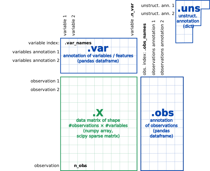
Figure 11: Schematic of the AnnData object with main components .X counts matrix, .obs metadata dataframe, and .var gene dataframe.
Image source: Scanpy Usage Principles

The 3 main slots in the scanpy object correspond with the 3 files used as input:

• .X is the counts matrix (matrix.mtx)
• .obs is the metadata for each cell (barcodes.tsv)
• .var is the metadata for each gene (features.tsv)

So let us start by loading in one of our samples, starting with the ctrl condition:

# Create scanpy object from ctrl sample
ctrl = sc.read_10x_mtx("data/ctrl_raw_feature_bc_matrix/")
ctrl

AnnData object with n_obs × n_vars = 737280 × 33538
    var: 'gene_ids', 'feature_types'
    layers: None (.X)

We can see from this callout that we have 737,280 cells (n_obs) and 33,538 genes (n_vars) which is clearly too many cells! So we can do some very low level filtration to remove any cells that we know are “empty”.

The pp.filter_cells() function specifies the minimum number of genes that need to be detected per cell. This argument will filter out poor quality cells that likely just have random barcodes encapsulated without any cell present. Usually, cells with less than 100 genes detected are not considered for analysis.

# Filter cells with less than 100 genes expressed
sc.pp.filter_cells(ctrl, min_genes = 100)
ctrl

AnnData object with n_obs × n_vars = 15688 × 33538
    obs: 'n_genes'
    var: 'gene_ids', 'feature_types'
    layers: None (.X)

We can see that we are now left with 15,688 cells.

At this point we do not have any information stored in our metadata, which is stored in the .obs slot of our AnnData object. Therefore, we will use the pp.calculate_qc_metrics() function:

# Calculate QC metrics for each cell
sc.pp.calculate_qc_metrics(ctrl,
                           percent_top = None,
                           log1p = False,
                           inplace = True)
ctrl.obs.head()

Table 5: First several rows of ctrl.obs

	n_genes	n_genes_by_counts	total_counts
AAACATACAATGCC-1	874	874	2344
AAACATACATTTCC-1	896	896	3125
AAACATACCAGAAA-1	725	725	2578
AAACATACCAGCTA-1	979	979	3261
AAACATACCATGCA-1	362	362	746

What do the columns of metadata mean?

• Sample or identity:
  • In Seurat: stored in orig.ident (defaults to "SeuratProject" unless set).
  • In scanpy: can be stored in obs["sample"] or another column you define.
• Number of UMIs per cell:
  • In Seurat: nCount_RNA
  • In scanpy: total_counts
• Number of genes detected per cell:
  • In Seurat: nFeature_RNA
  • In scanpy: n_genes

Reading in multiple samples with a for loop

In practice, you will likely have several samples that you will need to read in data for, and that can get tedious and error-prone if you do it one at a time. To import the data more efficiently, we can use a for loop. So instead, we will iterate over a series of commands for each of the inputs (samples) given and create scanpy/seurat objects.

for loop syntax

R

## DO NOT RUN
for (variable in input){
  command1
  command2
  command3
}

Python

## DO NOT RUN
for variable in input:
    command1
    command2
    command3

Today we will use it to iterate over the two sample folders and execute two commands for each sample as we did above for a single sample.

R

1. Read in the count data (Read10X()) and
2. Create the Seurat objects from the read in data (CreateSeuratObject())

sample_names <- c("ctrl", "stim")

# Empty list to populate seurat object for each sample
list_seurat <- list()

for (sample in sample_names) {
    # Path to data directory
    data_dir <- paste0("data/", sample, "_raw_feature_bc_matrix")

    # Create a Seurat object for each sample
    seurat_data <- Read10X(data.dir = data_dir)
    seurat_obj <- CreateSeuratObject(counts = seurat_data,
                                      min.features = 100,
                                      project = sample)

    # Save seurat object to list
    list_seurat[[sample]] <- seurat_obj
}

Breaking down the for loop

Step 1: Specify inputs

For this dataset, we have two samples and two associated folders that we would like to use as input to create the two Seurat objects:

• ctrl_raw_feature_bc_matrix
• stim_raw_feature_bc_matrix

We can specify these sample names in the input part for our for loop as elements of a vector using c(). We are assigning these to a variable and we can call that variable anything we would like (try to give it a name that makes sense). In this example, we called the variable sample.

During the execution of the above loop, sample will first contain the value “ctrl”, run through the commands all the way through to storing the seurat object as a list. Next, it will contain the value “stim” and once again run through all the commands. If you had 15 folders as input, instead of 2, the above code will run through 15 times, for each of your data folders.

To start, let us test out what happens if we print out what sample looks like and the associated data_dir path we specify.

sample_names <- c("ctrl", "stim")
# Empty list to populate seurat object for each sample
list_seurat <- list()

# Create each individual Seurat object
for (sample in sample_names) {
    print(sample)
    # Path to data directory
    data_dir <- paste0("data/", sample, "_raw_feature_bc_matrix")
    print(data_dir)
}

Step 2: Read in data for the input

We can continue our for loop by adding a line to read in data with Read10X():

## DO NOT RUN
        seurat_data <- Read10X(data.dir = data_dir)

Step 3: Create Seurat object from the 10X count data

Now, we can create the Seurat object by using the CreateSeuratObject() function, adding in the argument project, where we can add the sample name.

## DO NOT RUN
        seurat_obj <- CreateSeuratObject(counts = seurat_data, 
                                         min.features = 100, 
                                         project = sample)        

Step 4: Assign Seurat object to the list

The last command assigns the Seurat object created (seurat_obj) to the empty list that was initialized before the for loop. In this way, when we iterate and move on to the next sample in our input we will not overwrite the Seurat object created in the previous iteration:

## DO NOT RUN
        list_seurat[[sample]] <- seurat_obj
}

Python

1. Generate list of sample names
2. Read in the count data (sc.read_10x_mtx())
3. Filter out the very low quality data
4. Add the sample information to the metadata
5. Store AnnData to a dictionary (for later merging)

Go ahead and copy and paste the code below into your script and then run it.

# Create list of samples
sample_names = ["ctrl", "stim"]
# Initialize empty dictionary
dict_ad = dict()

# Loop over all the samples
for sample in sample_names:
    # Get the path for each sample
    path_data = f"data/{sample}_raw_feature_bc_matrix"
    print(path_data)

    # Load scanpy object
    ad = sc.read_10x_mtx(path_data)
    # Filter and add sample metadata
    sc.pp.filter_cells(ad, min_genes=100)
    ad.obs["sample"] = sample

    # Store scanpy object in the dictionary
    dict_ad[sample] = ad

data/ctrl_raw_feature_bc_matrix
data/stim_raw_feature_bc_matrix

Breaking down the for loop

Step 1: Specify inputs

For this dataset, we have two samples and two associated folders that we would like to use as input to create the two scanpy objects:

• ctrl_raw_feature_bc_matrix
• stim_raw_feature_bc_matrix

We can specify these sample names in the input part for our for loop as elements of a list. We are assigning these to a variable and we can call that variable anything we would like (try to give it a name that makes sense). In this example, we called the variable sample.

During the execution of the above loop, sample will first contain the value “ctrl”, run through the commands all the way through to storing the scanpy object as a list. Next, it will contain the value “stim” and once again run through all the commands. If you had 15 folders as input, instead of 2, the above code will run through 15 times, for each of your data folders.

# DO NOT RUN
## Loop over all the samples
for sample in sample_names:
    # Get the path for each sample
    path_data = f"data/{sample}_raw_feature_bc_matrix"
    print(path_data)

data/ctrl_raw_feature_bc_matrix
data/stim_raw_feature_bc_matrix

In our console, we saw that the path_data variable that was printed out twice corresponds with the location of where the sample input lives on our computer.

Step 2: Read in data for the input

We can continue our for loop by adding a line to read in data with sc.read_10x_mtx:

## DO NOT RUN
    # Load scanpy object
    ad = sc.read_10x_mtx(path_data)

Step 3: Filter cells and add sample column

We want to remove those low-quality cells (fewer than 100 genes expressed) and add a sample column to the metadata. Doing so will ensure that we can keep track of which cells originates from which sample.

## DO NOT RUN
    # Filter and add sample metadata
    sc.pp.filter_cells(ad, min_genes=100)
    ad.obs["sample"] = sample

Step 4: Assign scanpy object to the dictionary

The last command assignts the scanpy object created (ad) to the empty dictionary that was initialized before the for loop. In this way, when we iterate and move on to the next sample in our input we will not overwrite the scanpy object created in the previous iteration:

## DO NOT RUN
    # Store scanpy object in the dictionary
    dict_ad[sample] = ad

Now that we have created two objects for each of the samples, let’s take a quick look at the list. We should see that there are two single-cell objects in our list that correspond to each sample.

R

# List that contains ctrl and stim seurat objects
list_seurat

$ctrl
An object of class Seurat 
33538 features across 15688 samples within 1 assay 
Active assay: RNA (33538 features, 0 variable features)
 1 layer present: counts

$stim
An object of class Seurat 
33538 features across 15756 samples within 1 assay 
Active assay: RNA (33538 features, 0 variable features)
 1 layer present: counts

Python

# Dictionary that contains ctrl and stim scanpy objects
dict_ad

{'ctrl': AnnData object with n_obs × n_vars = 15688 × 33538
    obs: 'n_genes', 'sample'
    var: 'gene_ids', 'feature_types'
    layers: None (.X), 'stim': AnnData object with n_obs × n_vars = 15756 × 33538
    obs: 'n_genes', 'sample'
    var: 'gene_ids', 'feature_types'
    layers: None (.X)}

Next, we need to merge these objects together into a singular object. This will make it easier to run the QC steps for both sample groups together and enable us to easily compare the data quality for all the samples.

R

We can use the merge() function from the Seurat package to do this. Here, we also specify add.cell.id because the same cell IDs can be used for different samples so we add a sample-specific prefix to the cell IDs to ensure that they are unique.

# Create a merged Seurat object
merged_seurat <- merge(x = list_seurat[["ctrl"]],
                       y = list_seurat[["stim"]],
                       add.cell.id = c("ctrl", "stim"))

merged_seurat

An object of class Seurat 
33538 features across 31444 samples within 1 assay 
Active assay: RNA (33538 features, 0 variable features)
 2 layers present: counts.ctrl, counts.stim

What if I am merging more than two samples?

Seurat has the functionality to merge many samples together. You can do this quite easily by adding all sample objects to the y argument in a vector format. An example is provided below:

## DO NOT RUN
 merged_seurat <- merge(x = seurat_list[[1]],
                        y = seurat_list[2:length(seurat_list)],
                        add.cell.id = names(seurat_list))

However you may notice that when we look at our seurat object that we have 2 layers (count matrices) when it says:

2 layers present: counts.ctrl, counts.stim

This indicates that the matrices for each sample are being stored separately. Instead, we want to concatenate these together so that in the future when we run normalization, it is run on the entire dataset collectively. So, to create one counts matrix, that is not sample/batch specific, we run the JoinLayers() function.

# Concatenate the count matrices of both samples together
merged_seurat <- JoinLayers(merged_seurat)
merged_seurat

An object of class Seurat 
33538 features across 31444 samples within 1 assay 
Active assay: RNA (33538 features, 0 variable features)
 1 layer present: counts

Now that we’ve merged and joined the dataset as we wanted, we can verify that it looks correct. In the merged object’s metadata, we should see the rowname prefixes added by add.cell.id and the orig.ident values set during CreateSeuratObject with project = sample:

# Check that the merged object has the appropriate sample-specific prefixes
head(merged_seurat@meta.data)

Table 6: First several rows of a the merged_seurat@meta.data

	orig.ident	nCount_RNA	nFeature_RNA
ctrl_AAACATACAATGCC-1	ctrl	2344	874
ctrl_AAACATACATTTCC-1	ctrl	3125	896
ctrl_AAACATACCAGAAA-1	ctrl	2578	725
ctrl_AAACATACCAGCTA-1	ctrl	3261	979
ctrl_AAACATACCATGCA-1	ctrl	746	362
ctrl_AAACATACCTCGCT-1	ctrl	3519	866

# Check that the merged object has the appropriate sample-specific prefixes
tail(merged_seurat@meta.data)

Table 7: Last several rows of a the merged_seurat@meta.data

	orig.ident	nCount_RNA	nFeature_RNA
stim_TTTGCATGCGACAT-1	stim	620	295
stim_TTTGCATGCTAAGC-1	stim	1641	545
stim_TTTGCATGGGACGA-1	stim	1233	518
stim_TTTGCATGGTGAGG-1	stim	1084	469
stim_TTTGCATGGTTTGG-1	stim	818	432
stim_TTTGCATGTCTTAC-1	stim	1104	438

Python

We can use the anndata.concat() function to join both samples together. We specify that that we want the .values() of our dictionary - the actual scanpy object as the input for concatenating. Additionally, we want specify several arguments to ensure the merge is done correctly with:

Argument	Value	Description
join	"outer"	Keep the union of all genes across Scanpy objects; genes missing from a sample get filled with 0/NaNs.
label	"sample"	Create a new column in .obs called "sample" that records which input object each cell came from.
keys	sample_names	Values to put in the "sample" column, in the same order as the sample_names list.
index_unique	"_"	If cell IDs are duplicated across samples, make them unique by appending _{sample} (e.g., cell1_ctrl, cell1_stim).

Which we then store to a new variable named merged_adata that contains both ctrl and stim in one scanpy object.

# Pooling together the samples
merged_adata = anndata.concat(list(dict_ad.values()),
                              join = "outer",
                              label = "sample",
                              keys = sample_names,
                              index_unique = "_")

merged_adata

AnnData object with n_obs × n_vars = 31444 × 33538
    obs: 'n_genes', 'sample'
    layers: None (.X)

If we look at the metadata of the merged object we should be able to see the correct samples in the metadata:

merged_adata.obs.head()
merged_adata.obs.tail()

Table 8: First several rows of a the merged_adata.obs

	n_genes	sample
AAACATACAATGCC-1_ctrl	874	ctrl
AAACATACATTTCC-1_ctrl	896	ctrl
AAACATACCAGAAA-1_ctrl	725	ctrl
AAACATACCAGCTA-1_ctrl	979	ctrl
AAACATACCATGCA-1_ctrl	362	ctrl

Table 9: Last several rows of a the merged_adata.obs

	n_genes	sample
TTTGCATGCTAAGC-1_stim	545	stim
TTTGCATGGGACGA-1_stim	518	stim
TTTGCATGGTGAGG-1_stim	469	stim
TTTGCATGGTTTGG-1_stim	432	stim
TTTGCATGTCTTAC-1_stim	438	stim

Ultimately, we now have a merged object that contains all the cells from both ctrl and stim, as seen by looking at the first and last several cells. This means that we are all set to go for the next step, which is assessing the quality of our samples.

---

Next Lesson >>

Back to Schedule