Theory of Integration

This lesson introduces participants to the concepts involved in integrating single-cell RNA-seq datasets using canonical correlation analysis (CCA) and single cell Variational Inference (scVI). Participants will learn when integration is appropriate, how it aligns shared cell types across conditions and why evaluating data before integration is essential for accurate downstream analyses.

Keywords

R, Integration, CCA, scVI, Seurat, Scanpy, Mutual nearest neighbors

Approximate time: 90 minutes

Learning objectives

In this lesson, we will:

• Describe when integration is necessary
• Perform integration using either CCA or scVI to control for batch effects
• Plot UMAP representation of the cells

Overview of lesson

At this point in the analysis, we want to move onto the next step of annotating cells that are similar to one another (cell types). However, sometimes a detour is necessary to address technical effects due to differences between samples, conditions, modalities, or batches. In these cases, differences caused by unwanted variation may cause similar cells to be dissimilar. This integration is sometimes necessary in order to proceed with the analysis, but is not always required.

Figure 1: Overview of the single-cell RNA-seq workflow.

To integrate or not to integrate?

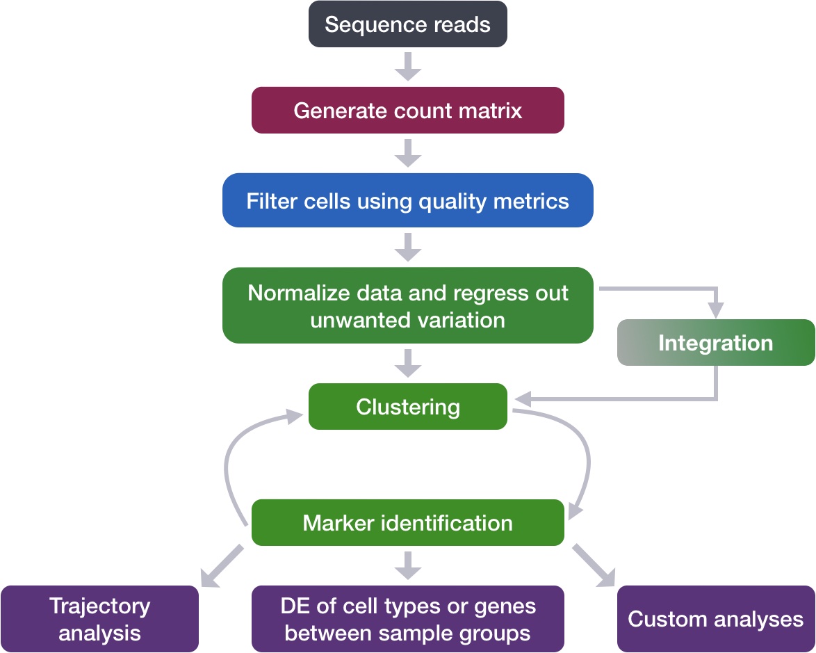
Generally, we always look at our clustering without integration before deciding whether we need to perform any alignment. It can be helpful to first run through clustering with samples from different sample classes together to see whether there are condition-specific clusters for cell types present in both conditions. Oftentimes, when clustering cells from multiple conditions there are condition-specific clusters and integration can help ensure the same cell types cluster together.

Do not just always perform integration because you think there might be differences - explore the data. If we had performed the normalization on both conditions together in a Seurat object and visualized the similarity between cells, we would have seen in our dataset there is condition-specific clustering.

Condition-specific clustering of the cells indicates that we need to integrate the cells across conditions to ensure that cells of the same cell type cluster together. If cells cluster by sample, condition, batch, dataset, modality, performing integration can help align cells across the groups to greatly improve the clustering and the downstream analyses.

Example scenarios for integration

• Different conditions (e.g. control and stimulated)

Figure 2: Example of condition-specific clustering and post-integration alignment using Seurat (control vs stimulated).

• Different datasets (e.g. scRNA-seq from datasets generated using different library preparation methods on the same samples)

Figure 3: Example of integrating multiple scRNA-seq datasets generated with different library preparation methods.

• Different batches (e.g. when experimental conditions make batch processing of samples necessary)

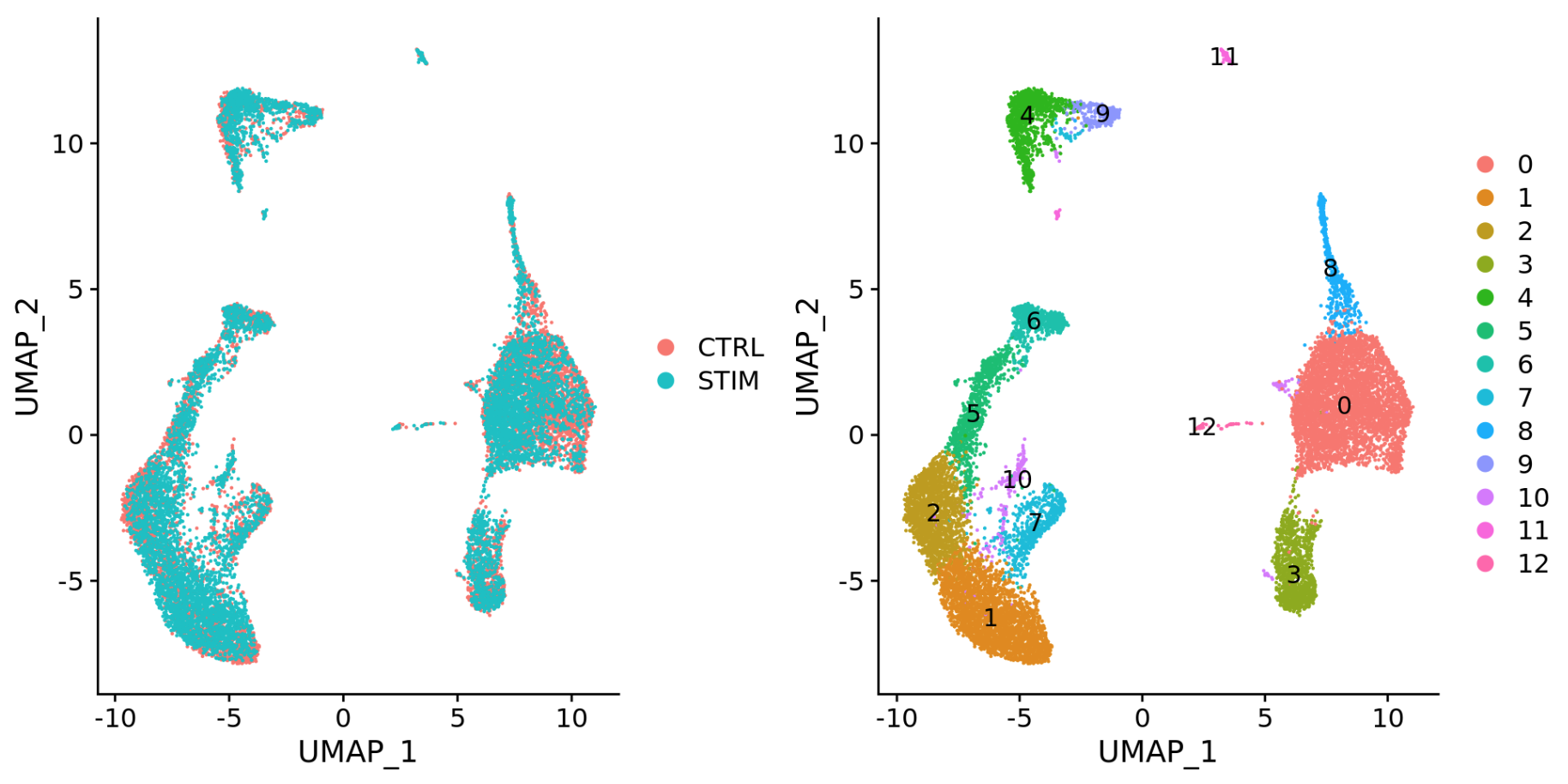
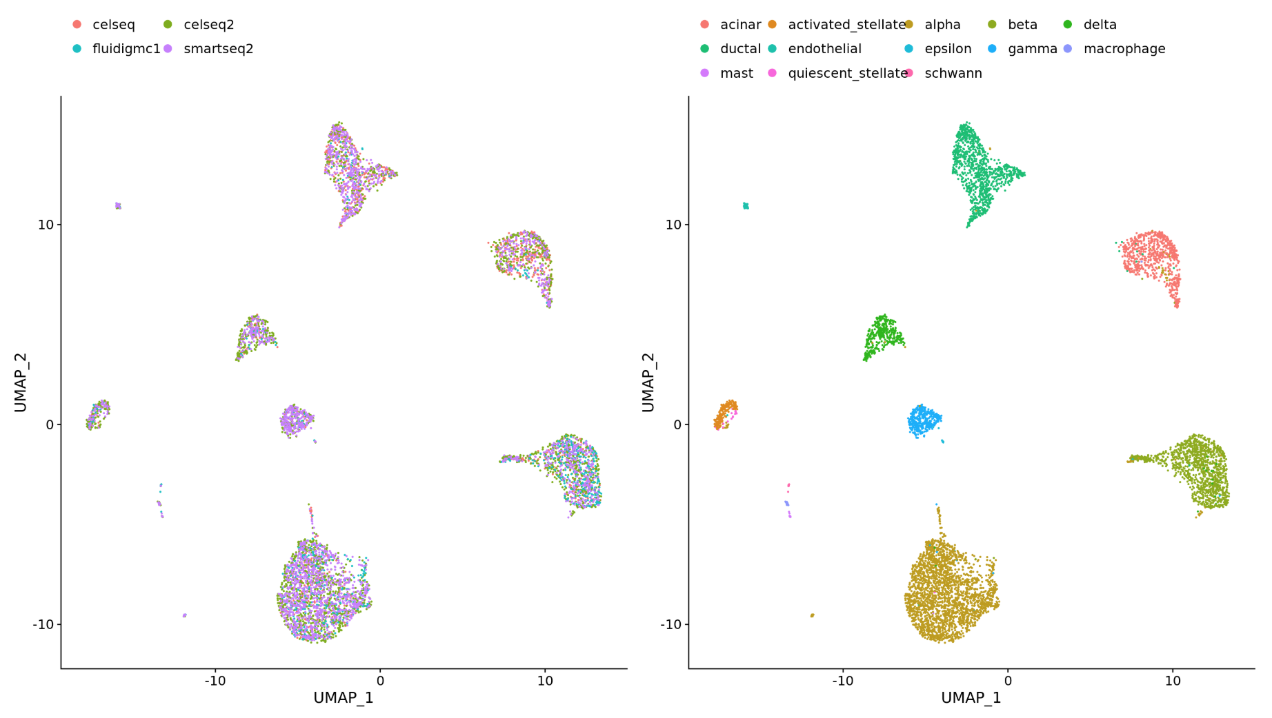
Why is it important that cells of the same cell type cluster together?

We want to identify cell states that are present in all samples/conditions/modalities within our dataset, and therefore would like to observe a representation of cells from both samples/conditions/modalities in every cluster. This will enable more interpretable results downstream (i.e. DE analysis, ligand-receptor analysis, differential abundance analysis…).

Integration in our dataset

So then how would you determine if integration is necessary?

One way is to return to our PCA embedding, where we noted that there was a clear divide amongst our cells based upon the sample condition - our only batch variable.

R

# Plot PCA colored by sample
DimPlot(seurat_phase,
        reduction = "pca",
        group.by = "sample")

Figure 4: Sample-specific clustering in PCA space, before integration.

Python

# Plot PCA colored by sample
sc.pl.pca(adata_phase,
           color="sample")

Figure 5: Sample-specific clustering in PCA space, before integration.

In this dataset, we know that the gene LYZ is a marker for monocytes. Even if the monocyte populations differ slightly between experimental conditions, we still expect monocytes from all batches to be biologically similar. Because of this, these cells should be considered comparable and should occupy the same region in the PCA embedding.

R

# Plot sample on PCA space
p_sample <- DimPlot(seurat_phase,
                    reduction = "pca",
                    group.by = "sample")

# Plot LYZ expression on PCA space
p_lyz <- FeaturePlot(seurat_phase,
                     reduction = "pca",
                     features = "LYZ")

p_sample + p_lyz

Figure 6: Expression of gene LYZ on the unintegrated PCA to show when integration is necessary.

In this lesson, we will cover the integration of our samples across conditions, which is adapted from the Seurat Guided Integration Tutorial.

Vignette without integration

Seurat has a vignette for how to run through the workflow from normalization to clustering without integration. Other steps in the workflow remain fairly similar, but the samples would not necessarily be split in the beginning and integration would not be performed.

Python

# Plot sample and LYZ expression on PCA space
sc.pl.embedding(adata_phase, 
                color=["sample", "LYZ"], 
                basis="pca")

Figure 7: Expression of gene LYZ on the unintegrated PCA to show when integration is necessary.

We can clearly see that there is a split in the grouping of monocytes that is driven by batch (sample).

Integration methods

There are many different integration methods that can be used to align single-cell RNA-seq datasets together. Some of the most popular methods include canonical correlation analysis (CCA) (Seurat based), single-cell Variational Inference (scVI) (scanpy based), and harmony. Here, we will discuss the underpinning logic of each method, before applying them practically in the next lesson.

Start with method for your programming language

This text is quite dense, so we recommend focusing on the method that suits the programming language you are working in first. scVI for python and CCA for R.

R: Canonical Correlation Analysis (CCA)

Integration is a powerful method that uses shared highly variable genes from each group to identify shared subpopulations across conditions or datasets Stuart and Butler et al. (2018). The goal of integration is to ensure that the cell types of one condition/dataset align with the same cell types of the other conditions/datasets (e.g. control macrophages align with stimulated macrophages).

The integration method that is available in the Seurat package utilizes the canonical correlation analysis (CCA); a method that expects “correspondences” or shared biological states among at least a subset of single cells across the groups. The result of this integration approach is a corrected data matrix for all datasets, enabling them to be analyzed jointly in a single workflow. To transfer information from a reference to query dataset, Seurat does not modify the underlying expression data, but instead projects continuous data across experiments.

The steps in the Seurat integration workflow are outlined in the figure below:

Figure 8: Overview of the Seurat integration workflow using canonical correlation analysis (CCA) and anchors. Source: Stuart & Butler et al., 2018

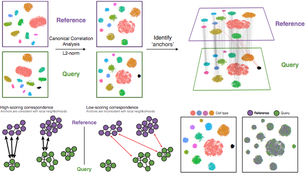
1. Identify shared variable genes:

Integration aims to take the matrix for each dataset (ctrl and stim) and identify correlated structures across them and align them in a common space. The shared highly variable genes from each dataset are used to form the intersection set, because they are the most likely to represent those genes distinguishing the different cell types present.

Each dataset can have a different number of cells, but must have the same number of genes.

2. Perform canonical correlation analysis (CCA):

Next, Seurat will jointly reduce the dimensionality of both datasets using diagonalized canonical correlation analysis (CCA) which is a form of PCA. Similar to principal components in PCA, the CCA will result in canonical correlation vectors. An L2-normalization is applied to the canonical correlation vectors, to use as input for the next step (identifying MNNs).

3. Find mutual nearest neighbors (MNNs) or anchors:

In this new shared low-dimensional space, Seurat will identify anchors or mutual nearest neighbors (MNNs) across datasets. These MNNs are pairs of cells that can be thought of as ‘best buddies’.

For each cell in one condition:

• The cell’s closest neighbor in the other condition is identified based on gene expression values - its ‘best buddy’.
• The reciprocal analysis is performed, and if the two cells are ‘best buddies’ in both directions, then those cells will be marked as anchors to ‘anchor’ the two datasets together.

4. Filter anchors to remove incorrect anchors:

Assess the similarity between anchor pairs by the overlap in their local neighborhoods (incorrect anchors will have low scores) - do the adjacent cells have ‘best buddies’ that are adjacent to each other? If not, these are removed the anchor list.

5. Integrate the conditions/datasets:

Using the anchors and corresponding scores the cell expression values are transformed, allowing for the integration of the conditions/datasets (different samples, conditions, datasets, modalities). For each cell in the dataset we now have an integrated value, but only for the variable features used for this analysis.

Neighborhoods and correction values

Transformation of each cell uses a weighted average of the two cells of each anchor across anchors of the datasets. Weights determined by cell similarity score (distance between cell and k nearest anchors) and anchor scores, so cells in the same neighborhood should have similar correction values.

If cell types are present in one dataset, but not the other, then the cells will still appear as a separate sample-specific cluster.

Reciprocal PCA

If there are a substantial number of cells that do not have a match between groups or there are a large number of cells to integrate, an alternative approach recommended by the Seurat vignette is reciprocal PCA (RPCA).

Python: single-cell Variational Inference (scVI)

scVI is a variational autoencoder that was published in 2018 by Lopez et. al to reduce technical noise and integrate disparate batches together. The method utilizes a variety of artificial intelligence methods to accomplish this task. To better understand the steps being used, we will first define what an autoencoder is, build upon the concept to define what variational autoencoders are, before lastly going through the scVI algorithm.

Autoencoders

Autoencoders are comprised of 3 main components:

• Encoder: Neural network where you supply inputs (image, count matrix) to create lower-dimension latent space.
• Latent space (bottleneck): Reduced representation of high-dimensional data (similar to PCA).
• Decoder: Neural network takes the latent space as input to reconstruct the original input.

Figure 9: Schematic of the architecture for an autoencoder, showcasing the encoder and decoder neural networks with the central latent space.
Image source: Lil’Log

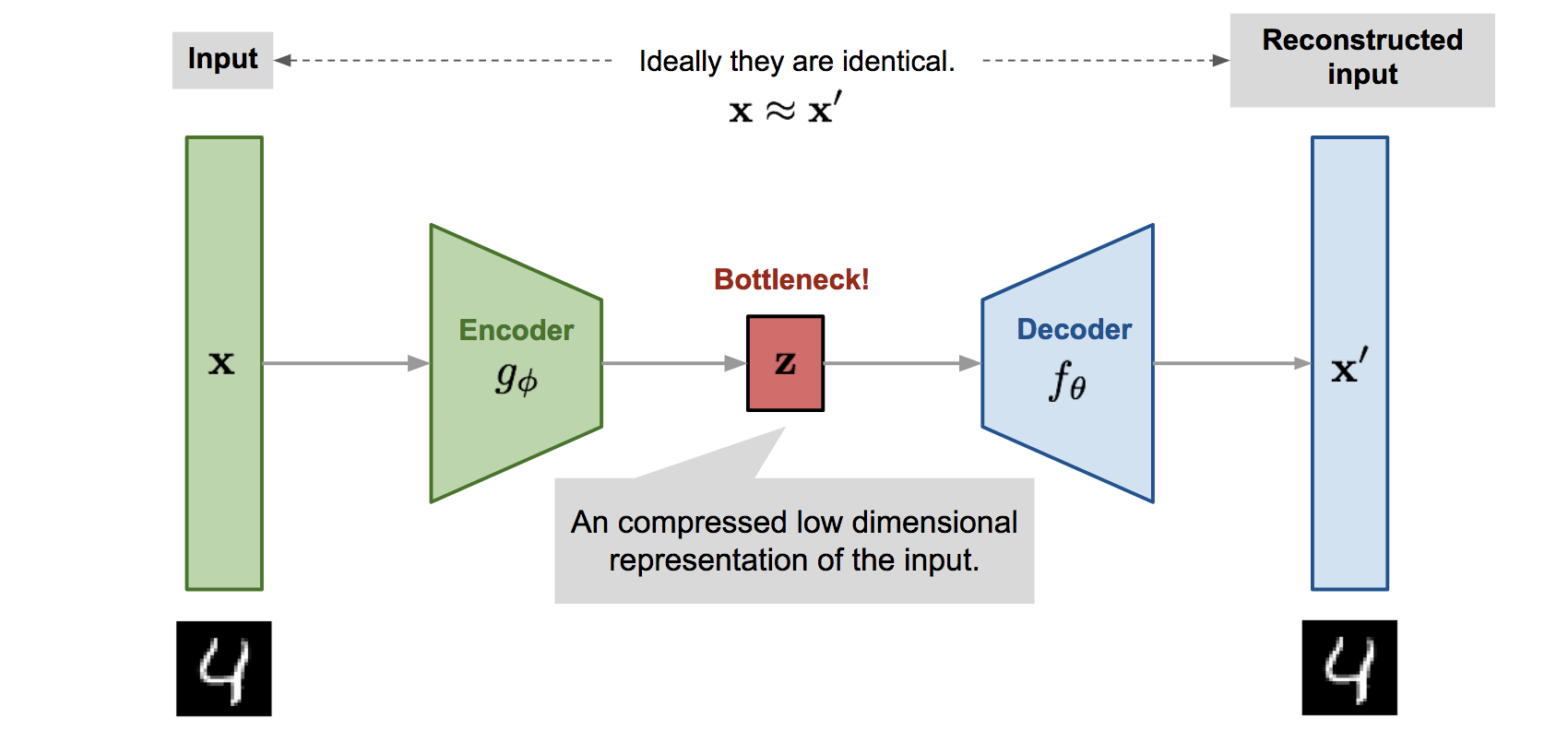
Ultimately, the goal of this method is to calculate the latent space. As we know what the input looks like, we also know what the expected output is as well. The encoder and decoder go back and forth to optimize the neural network, ultimately updating the values in the bottleneck until the output reconstructs the original input. This process repeats many times until the reconstruction is accurate.

Variational autoencoders

Variational autoencoders build upon these concepts by computing the mean (\(\mu\)) and variation (\(\sigma^{2}\)) for each input. Typically, this distribution is Gaussian.

Figure 10: Schematic of the architecture for a variational autoencoder.
Image source: Roger Yong

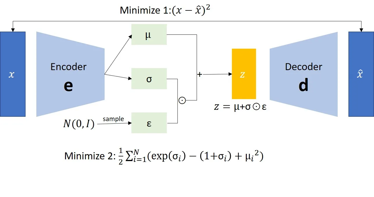
So at this point, we have multiple distributions to represent the original input. However, what we ultimately want is that low-dimensional representation (\(z\)) of our input. So the Gaussian distribution is randomly sampled and used as the latent space before being passed to the decoder.

scVI algorithm

As mentioned earlier, scVI is a variational autoencoder. The inputs supplied are the counts matrix as well as any batch (sample, donor, etc.) and unwanted variation (cell cycle phase, mitochondrial ratio, etc.).

Figure 11: Schematic of the scVI algorithm.
Image source: Lopez et al. (2018)

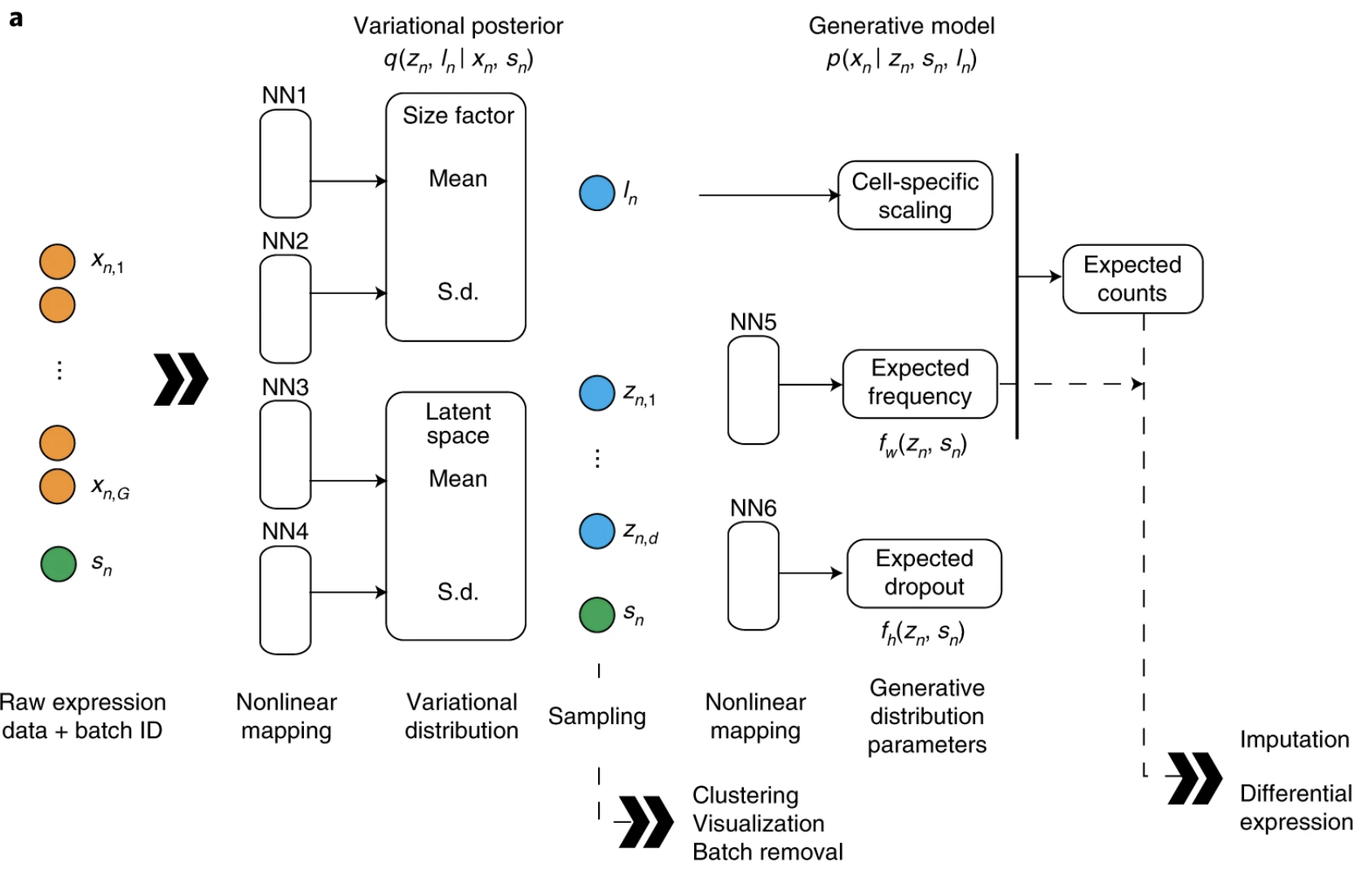
The broad steps of the scVI algorithm are as follows:

1. We assume there is a low-dimensional latent space \(z\) that can represent our dataset (similar to PCA).
2. The raw counts matrix and batch information are fed into the encoder, with the genes modelled as a Gaussian distribution of \(z\).
3. A latent representation \(z\) is sampled from this distribution and passed, along with the batch labels, into the decoder. The decoder tries to reconstruct the original counts, modelling gene expression as a zero-inflated negative binomial distribution.
4. The reconstructed counts are compared to the real counts, and the network weights are updated to minimise the difference. This is repeated many times until reconstruction is accurate.

• Encoder: counts + batch -> \(z\)
• Decoder: \(z\) + batch → reconstructed counts

5. Once the counts are reconstructed, the posterior mean of the \(z\) distribution for each cell is used as the latent space values for downstream analyses (clustering, UMAP, etc.).

---

Next Lesson >>

Back to Schedule