Contributors: Meeta Mistry, Upendra Bhattarai, Will Gammerdinger
Approximate time: 20 minutes
Learning Objectives
- Describe the workflow from sequence reads to peak calls
From sequence reads to peak calls
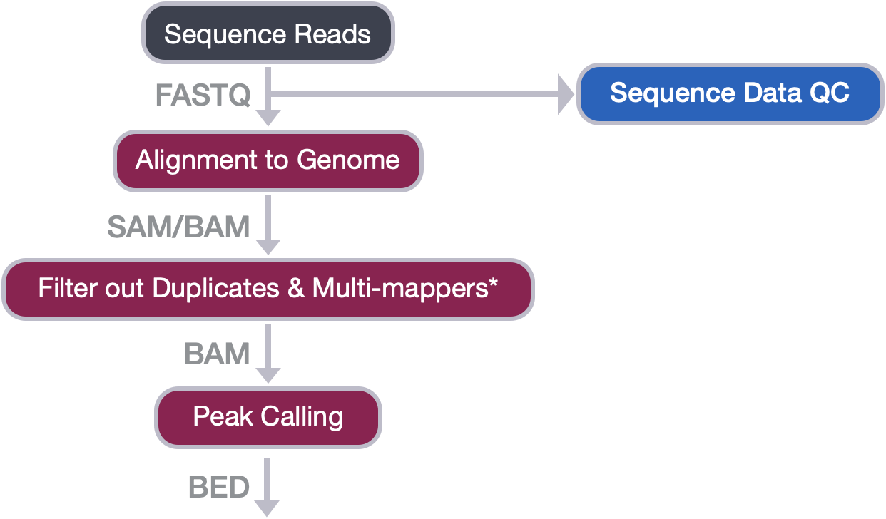
In this lesson, we will highlight the important steps involved in a typical workflow for the analysis of ChIP-seq or related data. If you are looking for more in-depth information on the background and theory for each step, we suggest looking at the Understanding chromatin biology using high throughput sequencing workshop materials.
NOTE: When starting out with your experiment, there are numerous quality control considerations at the bench when preparing your samples. We have highlighted some of the important points within this lesson. Investing time early in the experiment to ensure good quality samples will pay off with meaningful and reproducible results down the line.
Sequence Data QC
The raw sequence (FASTQ) files you obtain from the sequencing facility will first need to be assessed for quality. Here, we use the tool FastQC to look at metrics like base call quality, sequence duplication levels and overrepresented sequences.
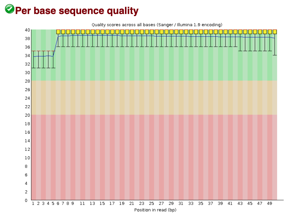
- Per Base Sequence Quality - This metric should stay mostly above a PHRED score of 30 and should have a smooth trajectory. It will oftentimes trail off with lower PHRED scores near the end of the read. Below is an image of a per base sequence quality analysis that has no concern features.
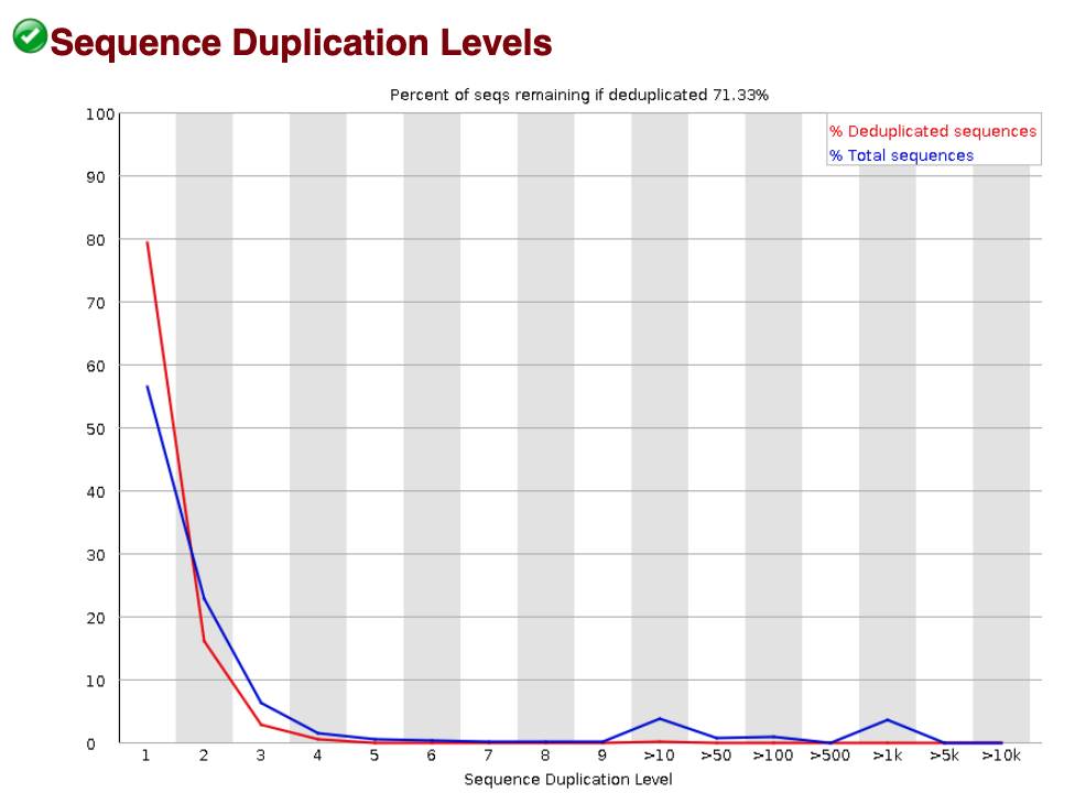
- Sequence Duplication Level - This metric should start high for the unique sequences and rapidly decrease. We remove duplicates later in the workflow, so we aren’t too concerned about their presence. However, if you see a high proportion of duplicated sequences, then the power to call peaks later may be impacted. Below is an image of a sequence duplication level analyis that has no concerning features.
- Overrepresented Sequences - This will flag reoccuring sequences in your dataset, which for some next-generation sequencing experiments could be problematic. However, for ChIP-seq experiments, we might expect to see some since we are enriching for particular sequences with immunoprecipitation. Targeted sequences don’t always show up in this statistic, so there’s not too much need to read too much into an target sequences presence or absence here.
At this stage we are flagging samples with values deviating from expected ranges. If the data doesn’t look reasonably clean at this point, it can make downstream processes more difficult and thus it may be grounds for removal of a sample from downstream analysis. Be sure to consult with your sequencing facility if you suspect there has been an issue in the sequencing.
More specific details on what we assess from the FastQC report can be found here.
Alignment to genome
Next, we take our reads and map them to the genome. There are a variety of tools used to align reads to a reference genome. For our workflow we use Bowtie2 for this task. The output from the alignment step will be a SAM/BAM file. If you are aligning to a high-quality reference genome (human/mouse/Drosophila), you should expect to see an alignment rate above 90%. If your alignment dips too far below this threshold, it could be the result of contamination.
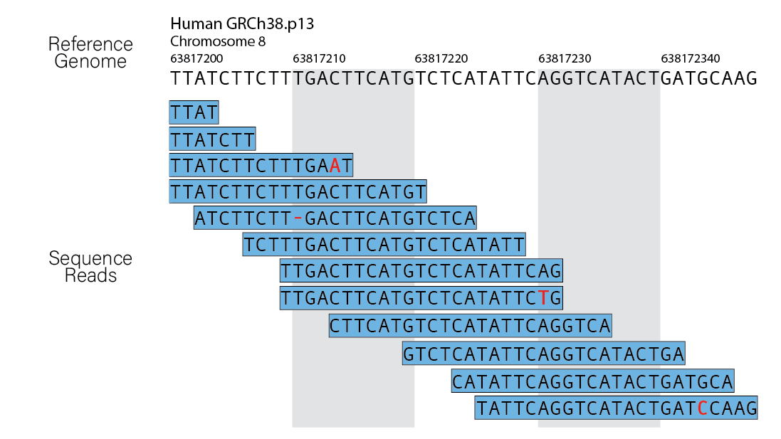
More details on this alignment procedure for ChIP-seq can be found here.
Filtering BAM files
The raw alignment output from Bowtie2 has a few issues that we will need to filter out for our analysis. These include:
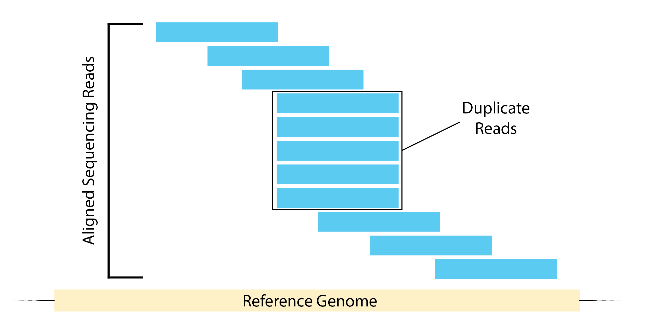
- Duplicate Reads - Duplicate reads are reads that map to the exact same location in the genome. Oftentimes, this is the result of overamplification of the input material when the input material is low. This can cause problems downstream by artificially enriching areas of protein binding. Alternatively, it could be the result of high sequencing depth or if your protein has limited binding sites. However, it is difficult to differentiate between these cases, so as a result we will remove duplicate reads.
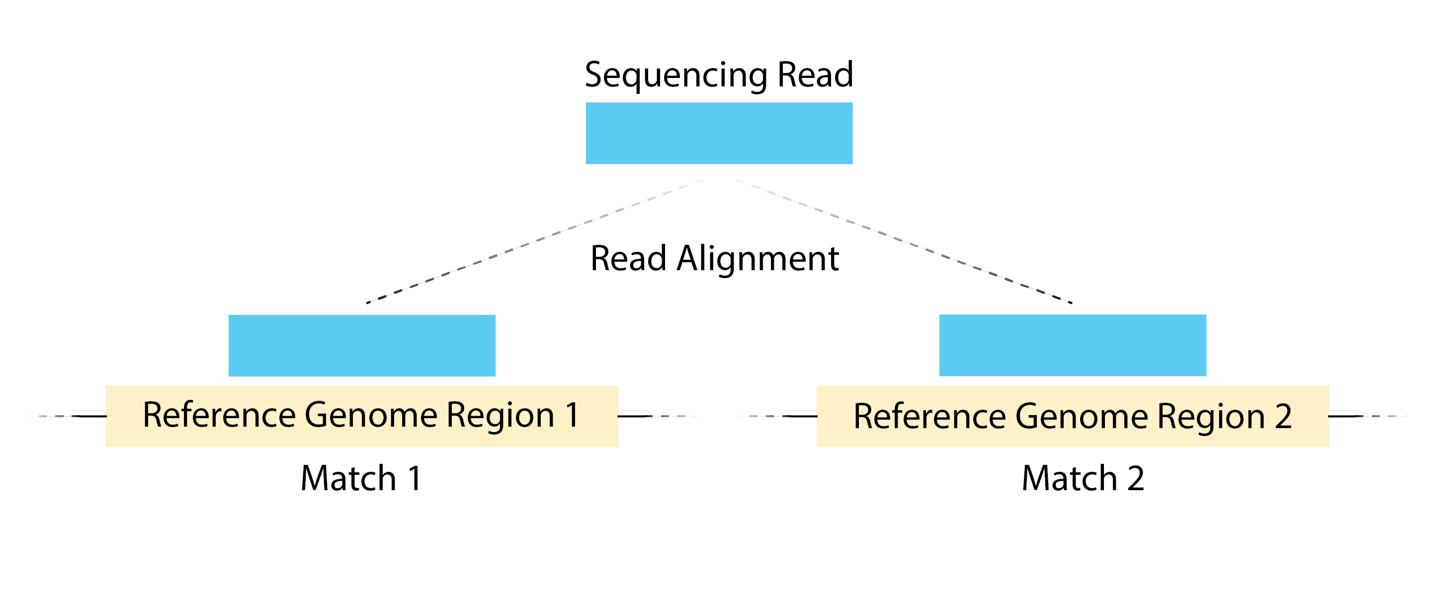
- Multimapping Reads - Reads can also map to multiple locations in the genome and we will want to remove these as well. If a read is matching to several different genomic regions, it creates ambiguity about the exact origin. Since peak calling algorithms typically rely on identifying regions with a high concentration of reads, multimapping reads can introduce noise and potentially lead to false positive peaks.
- Blacklisted Regions - Blacklisted regions represent artifact regions that tend to show artificially high signal (excessive unstructured anomalous reads mapping). These regions are often found at specific types of repeats such as centromeres, telomeres, and satellite repeats and typically appear uniquely mappable so simple mappability filters applied above do not remove them. The ENCODE and modENCODE consortia have compiled blacklists for various species and genome versions including human, mouse, worm, and fly. These blacklisted regions (coordinate files) can be filtered out from our alignment files before proceeding to peak calling. Alternatively, you can filter out peaks within blacklisted regions after you call your peaks. Either way, blacklisted regions should be removed from the dataset.
More details on this alignnment filtering procedure for ChIP-seq can be found here.
Peak calling
Peak calling, the next step in our workflow, is a computational method used to identify areas in the genome that have been enriched with aligned reads as a consequence of performing a ChIP-seq experiment.
For ChIP-seq experiments, what we observe from the alignment files is a strand asymmetry with read densities on the +/- strand, centered around the binding site. The 5’ ends of the selected fragments will form groups on the positive- and negative-strand. The distributions of these groups are then assessed using statistical measures and compared against background (input or IgG samples) to determine if the site of enrichment is likely to be a real binding site.
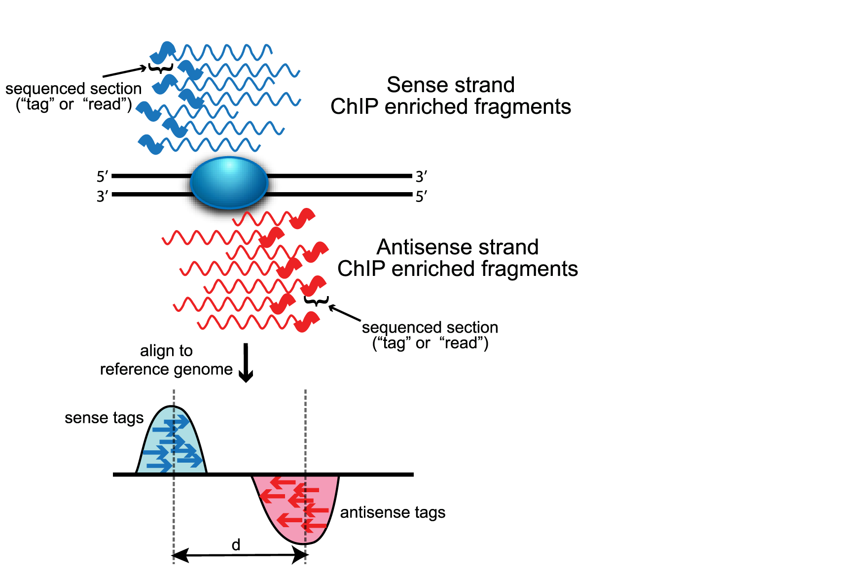
Image source: Wilbanks and Faccioti, PLoS One 2010
Similar to alignment algorithms, there are several options for peak calling algorithms and each offers their own strengths and can be dependent on the protein of interest. A more in-depth comparisons between peak calling algorithms can be found here. We used the tool MACS2 in order to call peaks in our dataset.
More details on this peak calling procedure for ChIP-seq as well as a more in-depth look on how MACS2 operates can be found here.
Additional resources on troubleshooting QC issues associated with ChIP-seq can be found here.
This lesson has been developed by members of the teaching team at the Harvard Chan Bioinformatics Core (HBC). These are open access materials distributed under the terms of the Creative Commons Attribution license (CC BY 4.0), which permits unrestricted use, distribution, and reproduction in any medium, provided the original author and source are credited.