Contributors: Mary Piper, Radhika Khetani, Meeta Mistry, Jihe Liu, Will Gammerdinger
Approximate time:
Learning Objectives
- Explain the components of a FASTQ file
- Evaluate the quality of the sequencing data using FastQC
Quality control of sequence reads
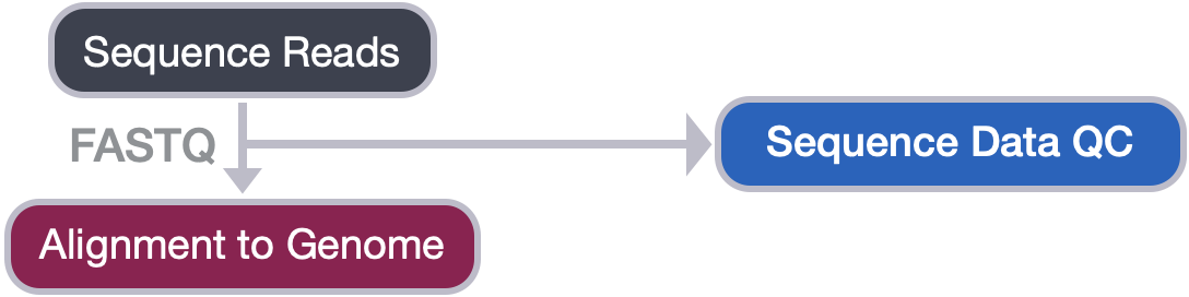
Now that we set up files and directory structure, we are ready for our ChIP-seq analysis. For any NGS analysis, the first step in the workflow is to evaluate the quality of the reads, prior to aligning them to the reference genome and downstream analyses.
Unmapped read data: FASTQ file format
The FASTQ file format is the defacto file format for sequence reads generated from next-generation sequencing technologies. This file format evolved from FASTA in that it contains sequence data, but also contains quality information. Similar to FASTA, the FASTQ file begins with a header line. The difference is that the FASTQ header is denoted by a @ character. For a single record (sequence read) there are four lines, each of which are described below:
| Line | Description |
|---|---|
| 1 | Always begins with ‘@’ and then information about the read |
| 2 | The actual DNA sequence |
| 3 | Always begins with a ‘+’ and sometimes the same info in line 1 |
| 4 | Has a string of characters which represent the quality scores; must have same number of characters as line 2 |
Let’s use the following read as an example:
@HWI-ST330:304:H045HADXX:1:1101:1111:61397
CACTTGTAAGGGCAGGCCCCCTTCACCCTCCCGCTCCTGGGGGANNNNNNNNNNANNNCGAGGCCCTGGGGTAGAGGGNNNNNNNNNNNNNNGATCTTGG
+
@?@DDDDDDHHH?GH:?FCBGGB@C?DBEGIIIIAEF;FCGGI#########################################################
As mentioned previously, line 4 has characters encoding the quality of each nucleotide in the read. The legend below provides the mapping of quality scores (Phred-33) to the quality encoding characters. Different quality encoding scales exist (differing by offset in the ASCII table), but note the most commonly used one is fastqsanger.
 Quality encoding: !"#$%&'()*+,-./0123456789:;<=>?@ABCDEFGHI
                   |         |         |         |         |
    Quality score: 0........10........20........30........40
Using the quality encoding character legend, the first nucelotide in the read (C) is called with a quality score of 31, and our Ns are called with a score of 2. As you can tell by now, this is a bad read.
Each quality score represents the probability that the corresponding nucleotide call is incorrect. This quality score is logarithmically based and is calculated as:
Q = -10 x log10(P), where P is the probability that a base call is erroneous
These probabaility values are the results from the base calling algorithm and dependent on how much signal was captured for the base incorporation. The score values can be interpreted as follows:
| Phred Quality Score | Probability of incorrect base call | Base call accuracy |
|---|---|---|
| 10 | 1 in 10 | 90% |
| 20 | 1 in 100 | 99% |
| 30 | 1 in 1000 | 99.9% |
| 40 | 1 in 10,000 | 99.99% |
| 50 | 1 in 100,000 | 99.999% |
| 60 | 1 in 1,000,000 | 99.9999% |
Therefore, for the first nucleotide in the read (C), there is less than a 1 in 1000 chance that the base was called incorrectly. However, for the end of the read, there is greater than 50% probabaility that the base is called incorrectly.
Assessing sequence read quality with FastQC
Now we understand what information is stored in a FASTQ file, the next step is to generate quality metrics for our sequence data.
FastQC provides a simple way to do some quality control checks on raw sequence data coming from high throughput sequencing pipelines. It contains a modular set of analyses, allowing us to have a quick glimpse of whether the data is problematic before doing any further analysis.
The main features of FastQC are:
- Imports data in FASTQ files (or BAM files)
- Evaluates the reads automatically and identifies potential issues in the data
- Generates a HTML-based quality report with graphs and tables
NOTE: Before we run FastQC, please check to make sure you are on a compute node. If not, please run the following
sruncommand to start an interactive session.$ srun --pty -p interactive -t 0-3:00 --mem 8G /bin/bashAn interactive session is very useful to test tools and workflows.
Running FastQC
When working in a cluster environment, you will find that generally many tools and software are pre-installed for your use. On the O2 cluster, these tools are available through the LMOD system. In order to see if the tool you are looking for exists as a module you can use the module avail command.
module avail fastqc
For more detailed information, we can use the module spider command:
$ module spider fastqc
Then we can decide on the version we would like to use and load the FastQC module:
$ module load fastqc/0.11.3
You should now see that the module is loaded:
$ module list
Once a module for a tool is loaded, it becomes directly available to you like any other basic UNIX command. That is, at the command prompt we just need to provide the name of the tool to use it. This is because the path to the executable file for FastQC has now been added to our $PATH variable. Check your $PATH variable to see whether or not you see a relevant path. Is it appended to the beginning or end? Do you see any additional paths added?
$ echo $PATH
Now we’re all set to run FastQC on one of our samples!
Before we do that we will create a fastqc directory under results, to store the FastQC output:
$ mkdir -p ~/chipseq_workshop/results/fastqc
To run FastQC we need to specify two arguments: one is the directory where the results are stored, which is indicated after the -o flag; another one is the file name of our FASTQ input. We will be using the two immunoprecipitated chip WT replicates as input:
$ fastqc -o ~/chipseq_workshop/results/fastqc/ ~/chipseq_workshop/raw_data/wt*chip.fastq.gz
NOTE: FastQC can also accept multiple files as input. In order to do this, you just need to separate each file name with a space. FastQC also recognizes multiple files with the use of wildcard characters.
You may have noticed that it takes a few minutes to run this single sample through FastQC. How can we speed it up?
We could run the program faster by making use of the multi-threading functionality of FastQC. This will enable us to run the same command, but have it be distributed across multiple cores instead of the single core we are using now. In order to specify multi-threading, we need to request those resources from the cluster. Our current interactive session is only using one core!
Exit the interactive session (now you should be at a “login node”), then start a new interactive session with 4 cores using the srun command.
$ exit  # exit the current interactive session

$ srun --pty -c 4 -p interactive -t 0-3:00 --mem 8G /bin/bash  # start a new one with 4 cpus (-c 6) and 8G RAM (--mem 8G)
Take a quick look at your $PATH variable. Is FastQC still listed in there? Since you have created a fresh new interactive there will be no modules loaded and your $PATH will only contain the default paths. Load the module again:
$ module load fastqc/0.11.3 # reload the module for the new session
Exercise:
-
We mentioned that FastQC has multi-threading capability, but have not provided information on how to use it. Since you are new to FastQC, you may need to explore the help documentation to get more information. Use the
--helpargument to check what arguments are available for FastQC.$ fastqc --helpOnce you have figured out what argument to use, run FastQC with 4 threads/cores.
Click here for solution
$ fastqc -o ~/chipseq_workshop/results/fastqc/ -t 4 ~/chipseq_workshop/raw_data/wt*chip.fastq.gz
-
Do you notice any difference in running time? Does multi-threading speed up the run?
Transfer FastQC Results
Let’s take a closer look at the files generated by FastQC:
$ ls -lh ~/chipseq_workshop/results/fastqc/
You should see two output files generated:
-
The first is an HTML file which is a self-contained document with various graphs embedded into it. Each of the graphs evaluate different quality aspects of our data, we will discuss in more detail in this lesson.
-
Alongside the HTML file is a zip file (with the same name as the HTML file, but with .zip added to the end). This file contains the different plots from the report as separate image files but also contains data files which are designed to be easily parsed to allow for a more detailed and automated evaluation of the raw data on which the QC report is built.
In order to view the HTML report in our browser, we need to transfer it over to our local laptop via FileZilla. (You should have downloaded this to your computer as part of the preparation instructions for class.) Follow the steps below to do so:
What is FileZilla?
FileZilla is a file transfer (FTP) client with lots of useful features and an intuitive graphical user interface. It basically allows you to reliably move files securely between two computers using a point and click environment. It has cross-platform compatability so you can install it on any operating system.
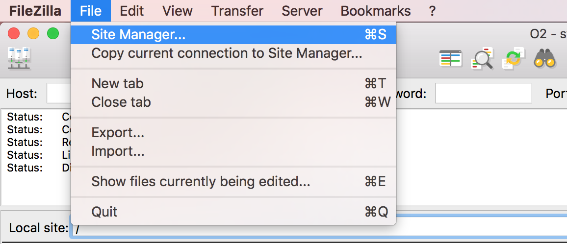
FileZilla - Step 1
Open FileZilla, and click on the File tab. Choose ‘Site Manager’.
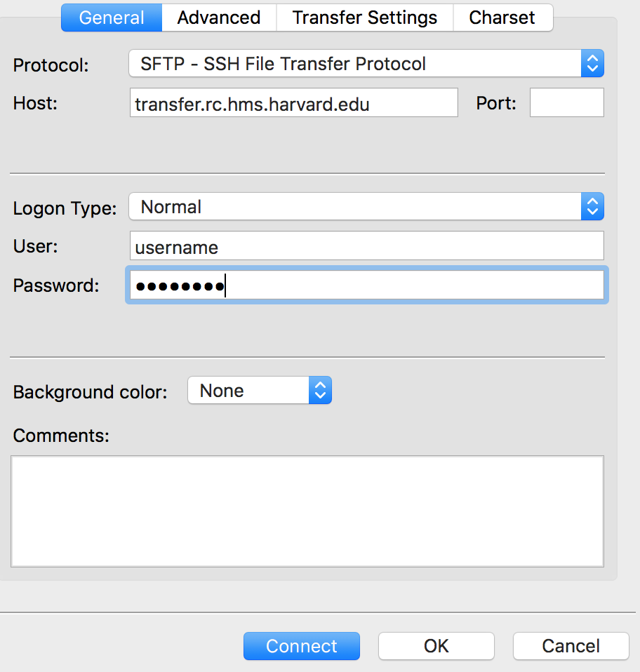
Filezilla - Step 2
Within the ‘Site Manager’ window, do the following:
- Click on ‘New Site’, and name it something intuitive (e.g. O2)
- Host: transfer.rc.hms.harvard.edu
- Protocol: SFTP - SSH File Transfer Protocol
- Logon Type: Normal
- User: training_account
- Password: password for training_account
- Click ‘Connect’
NOTE: While using the temporary training accounts on the O2 cluster, two-factor authentication IS NOT required. However, if you explore this lesson when using your personal account, two-factor authentication IS required.
In order to connect your laptop using FileZilla to the O2 cluster, follow steps 1-7 as outlined above. Once you have clicked ‘Connect’, you will receive a Duo push notification (but no indication in FileZilla) which you must approve within the short time window. Following Duo approval, FileZilla will connect to the O2 cluster. Additionally, each file transfer you carry out will also need Duo approval.
You will see messages in the top window panel, indicating whether or not you have successfully connected to O2. If this if your first time using FileZilla, we recommend that you take some time to get familiar with the basics of the interface. This tutorial is a helpful resource.
FileZilla Interface
You will see two panels in the interface. On the left hand side, you will see files from your laptop; on the right hand side, you will see your home directory on O2. Both panels have a directory tree at the top and a detailed listing of the selected directory’s contents underneath. On the right hand panel, navigate to where the HTML files are located on O2 ~/chipseq_workshop/results/fastqc/. Then on the left hand panel, select where you would like to copy those files to on your computer.
Copy the HTML report over by double clicking it or drag it over to the left hand side panel. Once finished, you can leave the FileZilla interface. Locate the HTML report on your computer, and open it up in a browser.
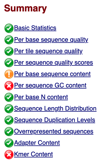
Interpreting the FastQC HTML report
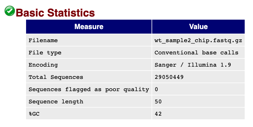
Now we can take a look at the various metrics generated by FastQC and assess the quality of our sequencing data!
Generally it is a good idea to take a look at basic statistics for the sample. Keep track of the total number of reads sequenced for each sample, and make sure the read length and %GC content is as expected.
On the left side of the report, a summary of all the modules is given. Don’t take the yellow “WARNING”s and red “FAIL”s too seriously - they should be interpreted as flags for modules to check out. Below we will discuss some of the relevant plots to keep an eye out for when using FastQC to assess ChIP-seq data.
Please note that the evaluation of FASTQC metrics will remain the same for CUT&RUN data, however there are minor differences when working with ATAC-seq data. Where appropriate, we have added pull-down sections on ATAC-seq.
Per base sequence quality
The Per base sequence quality plot is an important analysis module in FastQC for ChIP-seq; it provides the distribution of quality scores across all bases at each position in the reads. This information helps determine whether there are any problems during the sequencing of your data. Generally, we might observe a decrease in quality towards the ends of the reads, but we shouldn’t see any quality drops at the beginning or in the middle of the reads.
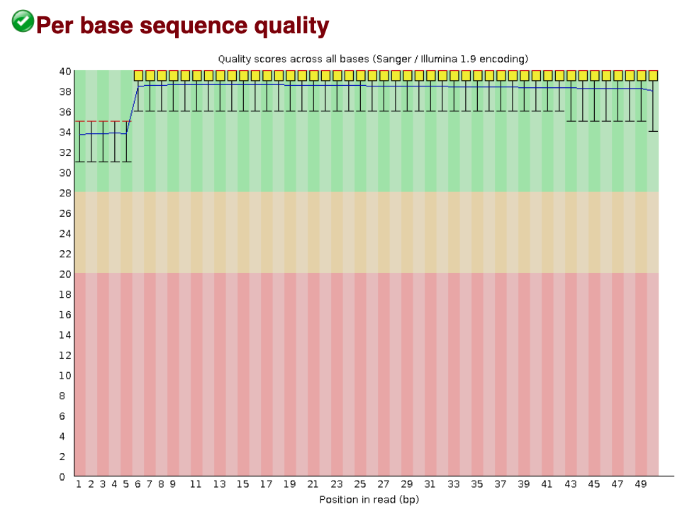
Based on the sequence quality plot of our sample, the majority of the reads have high quality. Particularly, the quality remains high towards the end of the read and we do not observe any unexpected quality drop in the middle of the sequence. If that happens, we will need to contact the sequencing facility for further investigation.
Sequence length distribution
The Sequence length distribution module generates a graph showing the distribution of fragment sizes in the file which was analysed. Most high-throughput sequencers generate reads of uniform length, and this will produce a simple graph showing a peak only at one size, but for variable length FastQ files this will show the relative amounts of each different size of sequence fragment.
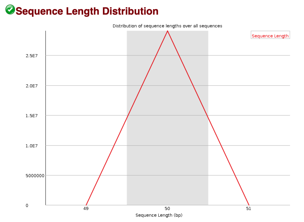
We observe a unique sequence length (50 bp) in our data, which is as expected. In some cases of ChIP-seq data, we have observed variable sequence lengths that is not due to the sequencer. Rather, this can be a result of the adapter removal in the previous steps suggesting that there was adapter contamination in your sample.
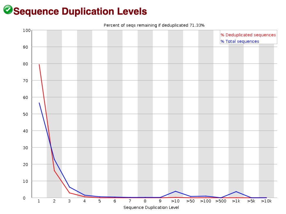
Sequence duplication levels
The Sequence duplication level plot indicates what proportion of your library corresponds to duplicates. Duplicates are typically removed in the ChIP-seq workflow (even if there is a chance that they are biological duplicates). Therefore, if we observe a large amount of duplication, the number of reads available for mapping and peak calling will be reduced. We don’t observe concerning duplication levels in our data.
Over-represented sequences
Over-represented sequences could come from actual biological significance, or biases introduced during the sequencing. With ChIP-seq, you expect to see over-represented sequences in the immunoprecipitation sample, because that’s exactly what you’re doing - enriching for particular sequences based on binding affinity. However, lack of over-represented sequences in FastQC report doesn’t mean you have a bad experiment. If you observe over-represented sequences in the input sample, that usually suggests some bias in the protocol to specific regions. Here, there is no over-represented sequences in our wt_sample2_chip sample.
Click here for Over-represented sequences in ATAC-seq
Since we are evaluating open regions and specific protein-DNA binding, and not enriching for very specific regions like in ChIP, we do not expect to see over-represented sequences for ATAC-seq data.
K-mer content
The Kmer content module examines whether there is positional bias for any small fragment of sequence. It measures the number of each 7-mer at each position in your library and then uses a binomial test to look for significant deviations from an even coverage at all positions. Any K-mers with positionally biased enrichment are reported and the top 6 most biased K-mers are additionally plotted to show their distribution.
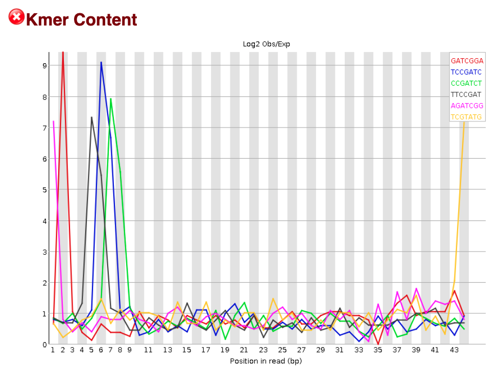
For our sample, we observe a significant amount of K-mer content and FastQC suggests a “Failure”. However, for ChIP-seq data a “Failure” of this metric is expected and is actually a sign of good signal in your data. Remember that the DNA sequences we have collected are from binding sites of our protein of interest. We would hope that there is some enrichment of K-mers amongst the binding sites (i.e shared motifs). We don’t expect this same result for the FastQC analysis of our input sample.
Click here for K-mer content in ATAC-seq
Since we are evaluating open regions and specific protein-DNA binding, and not enriching for very specific regions like in ChIP, we do not expect to see enrichment of specific kmers.
Conclusion
Based on the metrics and plots generated by FastQC, we have a pretty good quality sample to move forward with. Typically, you would generate these reports for all samples in your dataset and keep track of any samples that did not fare as well. We focused on the interpretation of selected plots that are particularly relevant for ChIP-seq, but if you would like to go through the remaining plots and metrics, FastQC has a well-documented manual page with more details (under the Analysis Modules directory) about all the plots in the report.
Additional resources
This lesson has been developed by members of the teaching team at the Harvard Chan Bioinformatics Core (HBC). These are open access materials distributed under the terms of the Creative Commons Attribution license (CC BY 4.0), which permits unrestricted use, distribution, and reproduction in any medium, provided the original author and source are credited.