# Set default assay to ADT
DefaultAssay(seurat_demux) <- "ADT"Protein Expression
Protein (ADT)
Normalization
Integration
Seurat
Normalizes antibody-derived tag (ADT) counts with CLR, runs PCA and UMAP on surface protein expression, and uses Harmony to correct library batch effects. Combines RNA and protein markers to annotate gut immune and stromal cell types, showing how protein overcomes RNA dropout for markers like CD4 and CD8.
Keywords
CITE-seq, antibody-derived tags (ADT), Harmony batch correction
Approximate time: 80 minutes
Learning objectives
In this lesson, we will:
- Normalize protein counts with CLR and exclude isotype controls
- Run PCA and UMAP on protein expression and correct library batch effects with Harmony
- Compare RNA and protein expression to see how each modality resolves cell types
- Annotate cell types using RNA and protein markers together
Overview of lesson
In this section, we will normalize the protein counts, reduce their dimensionality, and check whether the protein data alone separates our cells into sensible groups.
Protein expression (ADT)
Alongside RNA, each cell in our dataset was stained with a panel of 165 oligo-tagged antibodies, giving us a measure of surface protein abundance for every cell. Proteins are often the most direct readout of cell type, which allows us to infer cell identity from protein expression. For this project, many of the proteins were selected to identify immune cell types (e.g. CD3, CD4, CD8, CD19, HLA-DR).
Since this lesson focuses on the protein expression, we set our DefaultAssay to ADT to ensure that all calculations and visualizations are being done with the protein.
Isotype controls
Not every antibody in our panel targets a human protein. Isotype controls are antibodies of the same class as the real antibodies but with no target in human cells. Any counts they receive come from non-specific binding, so they tell us the level of background noise in each cell. They are useful for quality control, but they carry no biological signal, so we will exclude them from the downstream analysis.
Our panel contains the following nine isotype controls:
# Isotype control antibodies in the panel
isotypes <- c("ArmenianHamsterIgG",
"Mouse-IgG1-isotype", "Mouse-IgG2a-isotype", "Mouse-IgG2b-isotype",
"RatIgG1k", "RatIgG1l", "RatIgG2a", "Rat-IgG2b-isotype", "RatIgG2c")Before moving forward, we will first assess the expression levels of each of the isotype controls to confirm that there is little to no expression.
# Isotype control expression by HIV status
VlnPlot(seurat_demux,
group.by = "hiv_status",
features = isotypes,
assay = "ADT",
pt.size = 0)
We can see that there is practically zero expression of each of these isotypes, which confirms that we can proceed with our data as is.
Normalization
Antibody counts behave differently from RNA counts, which are typically log-normalized. Each antibody has its own background level, and a few highly abundant proteins can make up a large share of a cell’s counts. For this reason, we normalize with the centered log-ratio (CLR) transform, just as we did for the hashtags in the demultiplexing lesson. Setting margin = 2 normalizes each cell independently. As a result, each protein’s count is compared to the geometric mean of all the proteins in that cell.
# CLR normalization across proteins within each cell
seurat_demux <- NormalizeData(
seurat_demux,
normalization.method = "CLR",
margin = 2)
seurat_demuxAn object of class Seurat
36774 features across 34984 samples within 3 assays
Active assay: ADT (165 features, 0 variable features)
2 layers present: counts, data
2 other assays present: RNA, HTO
3 dimensional reductions calculated: pca_rna, harmony_rna, umap_rnaFeature selection
Recall that our protein panel is made up of 165 antibodies, which is a small number compared to the ~36,000 genes in the RNA assay. In a typical scRNA-seq workflow, this would be where we identify the top variable genes in the dataset. However, since there are so few proteins, we will instead use every protein except the isotype controls.
# Use all proteins except the isotype controls
adt_features <- setdiff(rownames(seurat_demux[["ADT"]]), isotypes)
VariableFeatures(seurat_demux) <- adt_features
length(adt_features)[1] 156We are left with 156 proteins, which we scale before running principal component analysis (PCA).
# Scale protein expression
seurat_demux <- ScaleData(seurat_demux)
seurat_demuxAn object of class Seurat
36774 features across 34984 samples within 3 assays
Active assay: ADT (165 features, 156 variable features)
3 layers present: counts, data, scale.data
2 other assays present: RNA, HTO
3 dimensional reductions calculated: pca_rna, harmony_rna, umap_rnaPCA
Principal Component Analysis (PCA) is a method that allows us to summarize and reduce the dimensions of our dataset to emphasize the variation and similarity of our data. Utilizing PCA, we are able to identify strong patterns in our dataset to group cells together.
Calculating PCA
Video on how PCA is calculated
For a more detailed explanation on PCA, please look over this lesson (adapted from StatQuests/Josh Starmer’s YouTube video). We also strongly encourage you to explore the video StatQuest’s video for a more thorough understanding.
Let’s say you are working with a single-cell RNA-seq dataset with 12,000 cells and you have quantified the expression of 20,000 genes. The schematic below demonstrates how you would go from a cell-by-gene matrix to principal component (PC) scores for each individual cell. This same principle applies for the ADT assay, except we use protein instead of genes.
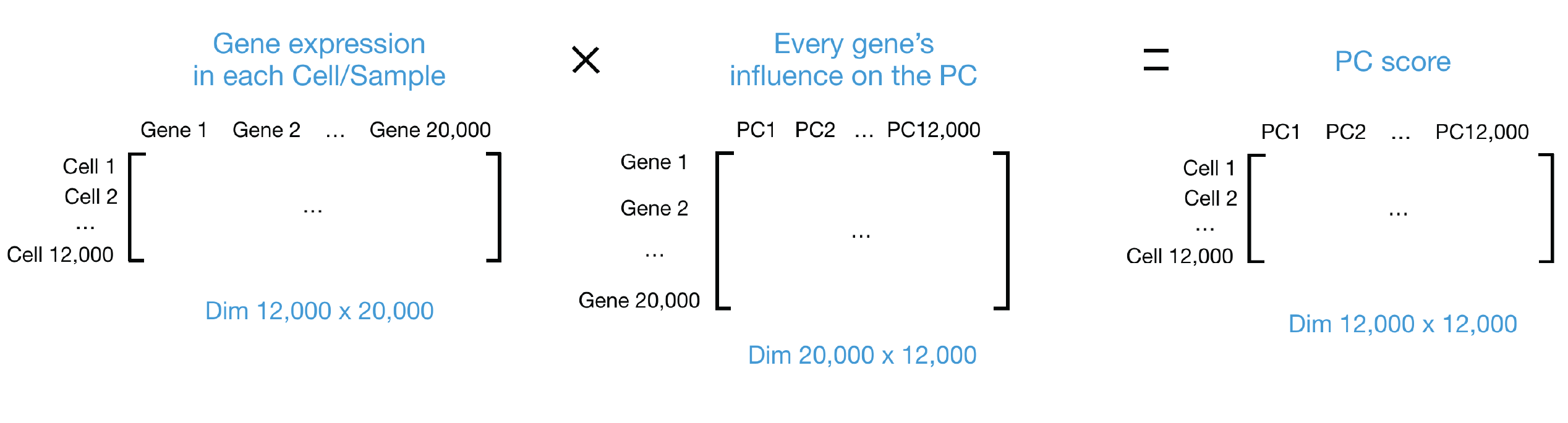
Now that we have a general idea of what the PCA calculation does, we can compute pca_adt using the RunPCA() function. At this step, we will also set the reduction.name to ensure that we can keep track of which assay a calculation was computed on.
# PCA on protein expression
seurat_demux <- RunPCA(
seurat_demux,
npcs = 30,
assay = "ADT",
reduction.name = "pca_adt",
reduction.key = "adtPC_",
verbose = FALSE,
seed.use = 123456789L)Visualizing PCA
Principal components analysis (PCA) stratifies the data by variance. Points closer together are more similar, and points further apart are more dissimilar. We can visualize the PCA results using DimPlot() to see whether any technical or biological variable is driving the separation of cells.
# Protein PCA by library and HIV status
DimPlot(seurat_demux,
group.by = c("orig.ident", "hiv_status"),
reduction = "pca_adt",
shuffle = TRUE)
The libraries are spread out along the first principal component: PT1 forms its own group at one end, PT4 sits at the other, and PT2 occupies its own region at the top of the plot. In this dataset, HIV status and library are confounded. Every PLWH cell comes from one of the three pooled libraries (PT1, PT2, and PT3). Therefore, we cannot yet tell how much of this separation is biology and how much is a technical difference between sequencing runs. We will keep an eye on this in the UMAP.
How many PCs should we use?
We computed 30 PCs, but the later steps (UMAP, Harmony, and clustering) use only the first 20. A common way to choose this number is an elbow plot, which shows the standard deviation explained by each PC. The point where the curve flattens out (the “elbow”) is where additional PCs stop adding much information.
# Elbow plot of protein PCs
ElbowPlot(seurat_demux,
ndims = 30,
reduction = "pca_adt")
The curve drops steeply over the first few PCs and flattens out between PCs 12 and 15. Using 20 PCs keeps everything up to the elbow with a small margin, without adding PCs that mostly capture noise.
PCA weights
We can additionally see which proteins have the highest weights (positive and negative) for each principal component. Ideally, we would hope to see cell type markers at this point.
# Top proteins for the first 5 PCs
print(seurat_demux[["pca_adt"]],
dims = 1:5, nfeatures = 5)adtPC_ 1
Positive: CD279, CD134, CD83, LOX-1, CD74
Negative: IgM, CD69, HLA-DR-DP-DQ, CD11a, CD8
adtPC_ 2
Positive: CD38, CD63, CD47, CD44, CD9
Negative: CD2, CD7, CD3, CD5, CD4
adtPC_ 3
Positive: CD2, CD69, CD7, CD45, CD3
Negative: HLA-DR-DP-DQ, CD22, HLA-DR, CD35, CD21
adtPC_ 4
Positive: CD63, CD38, CD48, CD49d, CD137
Negative: HLA-DR, HLA-DR-DP-DQ, CD22, CD35, CD150
adtPC_ 5
Positive: CD196, CD9, CD163, CD23, CD56
Negative: CD45, CD19, CD48, CD22, CD21 The later PCs look like cell type markers. adtPC_2 separates T cells (CD2, CD3, CD4, CD5, CD7). adtPC_3 and adtPC_4 are driven by B cell markers (CD21, CD22, CD35, HLA-DR). adtPC_1, however, mixes markers from many lineages, which fits with it separating libraries rather than cell types.
UMAP
UMAP takes the information from the top PCs and arranges the cells in two dimensions while trying to preserve local structure. Cells that are close together have similar protein expression based upon the values stored in the principal components. Bear in mind that the distances between clusters should not be over-interpreted.
First, we run UMAP directly on the uncorrected PCA.
# UMAP on uncorrected protein PCA
seurat_demux <- RunUMAP(
seurat_demux,
reduction = "pca_adt",
dims = 1:20,
reduction.name = "umap_adt_uncorrected",
reduction.key = "adtUncorrectedUMAP_",
verbose = FALSE,
seed.use = 123456789L)Now we can assess if the batch effect we identified in the PCA section is present in the UMAP.
# Protein UMAP before integration by library and HIV status
DimPlot(seurat_demux,
group.by = c("orig.ident", "hiv_status"),
reduction = "umap_adt_uncorrected",
shuffle = TRUE)
The batch effect is much clearer in the UMAP. Nearly all cells from PT2 and PT3 form a separate island, and PT1 occupies its own region instead of mixing with the HIV− libraries. Since we expect the same immune cell types to be present in every library, this is a strong sign that we need to run integration.
Harmony integration
If cells cluster by sample, batch, dataset, or modality, integration can greatly improve the clustering and downstream analyses. We “integrate” or “harmonize” the groups to overlay cells that share a common set of biological features. We use Harmony, which iteratively adjusts the principal components so that cells of the same type from different libraries are placed together.
In the case of our dataset, we will set group.by.vars = "orig.ident" to correct for differences between libraries.
# Correct protein PCs for library
seurat_demux <- RunHarmony(
seurat_demux,
group.by.vars = "orig.ident",
reduction.use = "pca_adt",
dims.use = 1:20,
reduction.save = "harmony_adt",
verbose = FALSE)This results in a batch-corrected dimensionality reduction, similar to PCA, which we call harmony_adt. With these corrected values, we can then run the UMAP algorithm again, but now on the corrected space to visualize how the cells appear to group together. If there is good overlap between the libraries, we then know that the integration step was successful.
# UMAP on corrected protein PCs
seurat_demux <- RunUMAP(
seurat_demux,
reduction = "harmony_adt",
dims = 1:20,
reduction.name = "umap_adt",
reduction.key = "adtUMAP_",
verbose = FALSE,
seed.use = 123456789L)
# Protein UMAP after integration, colored by library and HIV status
DimPlot(seurat_demux,
group.by = c("orig.ident", "hiv_status"),
reduction = "umap_adt",
shuffle = TRUE)
After Harmony, cells from every library are well mixed across the UMAP and no library forms its own island.
Over-correction
Because HIV status is confounded with library, correcting for library also removes any protein differences that are truly driven by HIV status. This is an acceptable tradeoff for visualizing cell types, but we should not use the integrated embedding to compare PLWH and HIV− cells.
Clustering
Now that we have an integrated protein embedding, we can group the cells into clusters based on their protein expression alone. Clustering is a graph-based approach that happens in two steps:
FindNeighbors(): Build a k-nearest neighbor graph, connecting each cell to the cells with the most similar protein expression. We use the Harmony-corrected PCs (harmony_adt) and the same 20 dimensions we used for the UMAP. We name the graphsnn_adtandsnn_adtso that they do not overwrite the RNA graphs.FindClusters(): Partition the shared nearest neighbor graph (snn_adt) into clusters. Settingalgorithm = 4uses the Leiden algorithm (Traag et al. 2019), which improves on the older Louvain algorithm by guaranteeing that the clusters it finds are well connected. The resolution sets the granularity: smaller values give fewer, larger clusters.
# Build the nearest neighbor graph on corrected protein PCs
seurat_demux <- FindNeighbors(
seurat_demux,
reduction = "harmony_adt",
dims = 1:20,
graph.name = c("nn_adt", "snn_adt"),
verbose = FALSE)
# Cluster the cells at a resolution of 0.8
seurat_demux <- FindClusters(
seurat_demux,
graph.name = "snn_adt",
resolution = 0.8,
algorithm = 4,
random.seed = 123456789L,
verbose = FALSE)Now that the clusters have been computed, we can visualize how well they group cells on the UMAP:
# ADT clusters and UMAP
DimPlot(seurat_demux,
group.by = "snn_adt_res.0.8",
reduction = "umap_adt",
label = TRUE)
Looking at a UMAP can be a bit subjective, so we encourage you all to use a variety of different visualizations to make decisions. For example, to assess how well the integration worked, we can plot the proportion of cells from orig.ident in each cluster as a bar plot:
# Barplot of proportion of cells in each cluster by orig.ident
ggplot(seurat_demux@meta.data) +
geom_bar(aes(x = snn_adt_res.0.8, fill = orig.ident),
position = position_fill(),
color = "black") +
theme_classic()
orig.ident.
From this, we can see that each library is represented in each cluster of our dataset, which is a more quantitative way to confirm that our integration step was successful.
Comparing RNA and ADT
The RNA assay was already run through the standard Seurat workflow, including the same integration, UMAP, and clustering steps. As a result, we now have two independent sets of clusters at the same resolution: one computed from RNA expression (snn_rna_res.0.8) and one from protein expression (snn_adt_res.0.8). Let’s start by plotting each set of clusters on the UMAP of its own modality, side by side.
# RNA clusters on the RNA UMAP
p_rna <- DimPlot(seurat_demux,
group.by = "snn_rna_res.0.8",
reduction = "umap_rna",
label = TRUE) +
ggtitle("RNA clusters")
# Protein clusters on the protein UMAP
p_adt <- DimPlot(seurat_demux,
group.by = "snn_adt_res.0.8",
reduction = "umap_adt",
label = TRUE) +
ggtitle("Protein clusters")
# Plot side by side
p_rna + p_adt
Even at the same resolution, the two modalities organize the cells quite differently. On the RNA UMAP, the clusters form well-separated islands, with clear gaps between the major groups. On the protein UMAP, most of the cells form one continuous structure. This difference comes from what each modality measures. RNA clustering uses 2,000 variable genes, which capture many cell type-specific programs, while protein clustering uses our panel of 156 surface markers. Cells that share most of their surface markers end up close together in protein space, even if their transcriptomes are distinct.
The RNA clusters were pre-computed at a resolution of 0.8 and are stored in the snn_rna_res.0.8 column. A useful check is to color the protein UMAP by these RNA clusters: if both modalities capture the same cell types, each RNA cluster should occupy its own region of the protein UMAP.
# RNA clusters on the protein UMAP
DimPlot(seurat_demux,
group.by = "snn_rna_res.0.8",
reduction = "umap_adt",
label = TRUE)
The RNA clusters do not map one-to-one onto regions of the protein UMAP. Some RNA clusters stay together, while others are spread across or merged with their neighbors. This is largely due to the proteins in our panel: they were chosen to distinguish immune populations, so cell types without matching markers on the panel look alike in protein space. As a result, the protein expression alone is not capable of identifying populations such as epithelial cells. This shows that each modality captures different information about a cell, which is why combining them can give a more complete picture than either one alone.
Cell typing
Now that we have both RNA and protein measurements for every cell, we can use them together to assign a cell type to each RNA cluster. We use a set of known marker genes for the cell populations expected in the human gut. For many of the immune populations, our antibody panel also contains a matching protein, which gives us a second, independent line of evidence.
| Cell type | Marker genes (RNA) | Marker proteins (ADT) |
|---|---|---|
| CD4 T | CD3E, CD4, IL7R, CD40LG | CD3, CD4 |
| CD8 T | CD8A, CD8B, GZMK | CD3, CD8 |
| B naive | MS4A1, IGHD, TCL1A, FCER2 | CD19, CD20, IgD |
| B memory | CD27, TNFRSF13B, AIM2 | CD19, CD20, CD27 |
| B proliferating | MKI67, TOP2A, AICDA, RGS13 | CD19, CD20 |
| Plasma cell - IgA | JCHAIN, IGHA1, IGHA2, MZB1 | CD27, CD38 |
| Plasma cell - IgG | IGHG1, IGHG3, IGHG4 | CD27, CD38 |
| CD14 monocytes | CD14, LYZ, S100A8, FCN1 | CD14, HLA-DR |
| NK | NKG7, GNLY, KLRD1, NCAM1 | CD56 |
| Mast | TPSAB1, CPA3, KIT, MS4A2 | |
| Epithelial | EPCAM, KRT8, KRT20, CDH1 | |
| Colonic subepithelial | PDGFRA, F3, BMP4, SOX6 | |
| Endothelial | PECAM1, VWF, CDH5, PLVAP | CD31 |
| Enteric glia | PLP1, S100B, SOX10, CDH19 | |
| Myenteric ganglia | ELAVL4, PHOX2B, RET, SNAP25 | |
| Myofibroblast | ACTA2, TAGLN, MYH11, DES |
Notice that the protein column is empty for many non-immune cell types. The antibody panel was designed to profile immune cells, so for the epithelial and stromal populations we will have to rely on RNA alone.
Identifying CD4+ and CD8+ T cells
Having protein expression can be really valuable when it comes to identifying cell types in your dataset. When working with single-cell RNA-seq, you must always be cognizant of dropout. This is a common problem in scRNA-seq, where genes that should be expressed are not captured in the experiment. Protein expression suffers much less from dropout, which makes it a valuable resource for confidently assigning cell type identities. To showcase the differences between protein and RNA, we can compare expression of the same gene/protein in both assays. In this case, we will use CD4 and CD8 as our markers of interest as they are markers for CD4+ and CD8+ T cells respectively.
To see this, we plot the RNA and protein expression of CD4 and CD8 side by side on the RNA UMAP. Since the same feature name (e.g. CD4) exists in both the RNA and ADT assays, we add the assay key as a prefix (rna_ or adt_) to tell Seurat which one to plot.
# CD4 and CD8 expression from RNA and protein
Idents(seurat_demux) <- "snn_rna_res.0.8"
FeaturePlot(seurat_demux,
features = c("rna_CD4", "rna_CD8A",
"adt_CD4", "adt_CD8"),
reduction = "umap_rna",
order = TRUE,
label = TRUE,
ncol = 2)
The two modalities tell a consistent story, but with different clarity. We can see that the expression of CD4 and CD8 is more sparse when looking at the RNA expression. In contrast, cells show more uniform expression in the ADT assay. This is much more evident when we look at a violin plot of clusters 1, 3, and 11 where our T cells are located.
# Violin plot of CD4 and CD8 expression in T cell clusters
VlnPlot(seurat_demux,
features = c("rna_CD4", "rna_CD8A",
"adt_CD4", "adt_CD8"),
idents = c(1, 3, 11),
ncol = 2,
pt.size = 0)
From the violin plot, we can see that the majority of cells have near 0 expression of CD4 and CD8 RNA. In contrast, the proteins are detected in many more cells. This makes it much easier to confidently assign cell type identities to clusters 1 and 11 as CD4+ T cells as well as cluster 3 as CD8+ T cells.
Assigning cell types
Using the marker genes and proteins, we assigned a cell type to each of the RNA clusters. We typically recommend using multiple markers as the justification for how a cell type was identified. Knowing top or known marker genes/proteins is the best way to identify each population. In the dropdown, we show the dotplot of the markers referenced in the earlier table.
DotPlot of top markers
Here we plot the marker genes, focusing on the RNA expression.
# Marker genes for each cell type
markers_gut <- list(
"CD4 T" = c("CD3E", "CD4", "IL7R", "CD40LG"),
"CD8 T" = c("CD8A", "CD8B", "GZMK"),
"B naive" = c("MS4A1", "IGHD", "TCL1A", "FCER2"),
"B memory" = c("CD27", "TNFRSF13B", "AIM2"),
"B proliferating" = c("MKI67", "TOP2A", "AICDA", "RGS13"),
"Plasma cell - IgA" = c("JCHAIN", "IGHA1", "IGHA2", "MZB1"),
"Plasma cell - IgG" = c("IGHG1", "IGHG3", "IGHG4"),
"CD14 monocytes" = c("CD14", "LYZ", "S100A8", "FCN1"),
"NK" = c("NKG7", "GNLY", "KLRD1", "NCAM1"),
"Mast" = c("TPSAB1", "CPA3", "KIT", "MS4A2"),
"Epithelial" = c("EPCAM", "KRT8", "KRT20", "CDH1"),
"Colonic subepithelial" = c("PDGFRA", "F3", "BMP4", "SOX6"),
"Endothelial" = c("PECAM1", "VWF", "CDH5", "PLVAP"),
"Enteric glia" = c("PLP1", "S100B", "SOX10", "CDH19"),
"Myenteric ganglia" = c("ELAVL4", "PHOX2B", "RET", "SNAP25"),
"Myofibroblast" = c("ACTA2", "TAGLN", "MYH11", "DES"))
DotPlot(seurat_demux, markers_gut,
group.by = "snn_rna_res.0.8",
assay = "RNA") +
theme(axis.text.x = element_text(angle = 90, vjust = 0.5, hjust = 1),
strip.text.x = element_text(angle = 90, hjust = 0))
We can do the same with the marker proteins, this time using the ADT assay. DotPlot() can only show each feature once, so proteins shared by several cell types (e.g. CD3 for all T cells) are grouped together:
# Marker proteins for each cell type
markers_gut_adt <- list(
"T cells" = c("CD3"),
"CD4 T" = c("CD4"),
"CD8 T" = c("CD8"),
"B cells" = c("CD19", "CD20"),
"B naive" = c("IgD"),
"B memory / Plasma" = c("CD27", "CD38"),
"CD14 monocytes" = c("CD14", "HLA-DR"),
"NK" = c("CD56"),
"Endothelial" = c("CD31"))
DotPlot(seurat_demux, markers_gut_adt,
group.by = "snn_rna_res.0.8",
assay = "ADT") +
theme(axis.text.x = element_text(angle = 90, vjust = 0.5, hjust = 1),
strip.text.x = element_text(angle = 90, hjust = 0))
Notice that CD56, our NK cell protein marker, is highest in cluster 18 rather than in the NK cells (cluster 6). Cluster 18 expresses the enteric glia genes PLP1, SOX10, and CDH19, and enteric glia also express CD56 (NCAM1) on their surface. This is a good reminder that a single protein is rarely specific to one cell type, so we should always look at several markers, across both modalities, before assigning a label.
Once we are confident in how we want to map the clusters to cell types, we create a named list of cell type labels. We will be using this list to rename our cells so that they are labelled by cell type rather than cluster in the next step.
# Cluster to cell type labels
celltype_labels <- list(
"1" = "CD4 T",
"2" = "Plasma cell - IgA",
"3" = "CD8 T",
"4" = "B memory",
"5" = "Plasma cell - IgA",
"6" = "NK",
"7" = "Plasma cell - IgA",
"8" = "Plasma cell - IgA",
"9" = "Colonic subepithelial",
"10" = "B naive",
"11" = "CD4 T",
"12" = "Plasma cell - IgG",
"13" = "B proliferating",
"14" = "Colonic subepithelial",
"15" = "CD14 monocytes",
"16" = "Plasma cell - IgA",
"17" = "Endothelial",
"18" = "Enteric glia",
"19" = "Mast",
"20" = "Myofibroblast"
)We also define the color palette used in the original publication:
# Color for each cell type
pal_gut <- c(
"CD4 T" = "#F4766E",
"CD8 T" = "#E78526",
"B naive" = "#FCDE13",
"B memory" = "#D8E025",
"B proliferating" = "#8FC740",
"Plasma cell - IgA" = "#0C964A",
"Plasma cell - IgG" = "#106B39",
"CD14 monocytes" = "#1CBAE9",
"NK" = "#1374BC",
"Mast" = "#273B90",
"Epithelial" = "#808EC5",
"Colonic subepithelial" = "#A780BB",
"Endothelial" = "#E16CA8",
"Enteric glia" = "#C79A6B",
"Myenteric ganglia" = "#AB7D52",
"Myofibroblast" = "#754D29"
)To apply the labels, we set the identities of our cells to the RNA clusters and use RenameIdents() to replace each cluster number with its cell type. We then store the result in a new celltype column in the metadata, ordering (factoring) the cell types to match the palette.
# Set idents to the RNA clusters
Idents(seurat_demux) <- "snn_rna_res.0.8"
# Rename the clusters and keep the labels in the metadata
seurat_demux <- RenameIdents(seurat_demux, celltype_labels)
seurat_demux$celltype <- Idents(seurat_demux)
seurat_demux$celltype <- factor(seurat_demux$celltype, levels = names(pal_gut))Finally, we can visualize our cell type annotations on both the RNA and protein UMAPs.
# Cell types on the RNA UMAP
p1 <- DimPlot(seurat_demux,
group.by = "celltype",
reduction = "umap_rna",
label = TRUE,
cols = pal_gut) +
NoLegend() +
ggtitle("UMAP RNA")
# Cell types on the protein UMAP
p2 <- DimPlot(seurat_demux,
group.by = "celltype",
reduction = "umap_adt",
label = TRUE,
cols = pal_gut) +
ggtitle("UMAP ADT")
p1 | p2
On the RNA UMAP, each cell type forms a distinct group, which is expected since the clusters were defined on RNA. On the protein UMAP, immune populations with strong surface markers in our panel, such as the CD4 T cells, occupy their own regions. Other populations are more mixed, likely due to the lack of strong marker proteins for those cells.
We can also take this opportunity to count how many cells belong to each cell type.
# Count number of cells
table(seurat_demux$celltype)
CD4 T CD8 T B naive
6105 3896 1634
B memory B proliferating Plasma cell - IgA
3598 500 12287
Plasma cell - IgG CD14 monocytes NK
676 491 2469
Mast Epithelial Colonic subepithelial
254 0 2289
Endothelial Enteric glia Myenteric ganglia
366 277 0
Myofibroblast
142 Notably, two of the populations from our marker table, epithelial cells and myenteric ganglia, have 0 cells because none of the RNA clusters matched them. These cells may become more apparent once we incorporate the ATAC-seq information in future lessons.
Protein vs RNA Expression
Earlier, we saw that CD4 protein marks the CD4 T cells much more clearly than the CD4 transcript. To look at this more closely, we can compare the RNA and protein expression of CD4 in each individual CD4 T cell.
First, we use FetchData() to pull the RNA and protein values for CD4, along with the cell type labels, into a dataframe. As before, the rna_ and adt_ prefixes tell Seurat which assay to take each value from.
# RNA and protein expression of CD4 for each cell
df_cd4 <- FetchData(seurat_demux,
vars = c("rna_CD4", "adt_CD4", "celltype"),
layer = "data")
head(df_cd4)ADT and RNA expression of CD4 for each cell.
| rna_CD4 | adt_CD4 | celltype | |
|---|---|---|---|
| B351A_AAACAGCCACAGGATG-1 | 2.238069 | 1.4980466 | CD8 T |
| B351A_AAACCGCGTCCCGAAG-1 | 0.000000 | 0.0000000 | Plasma cell - IgA |
| B351A_AAACGGATCCCGAACA-1 | 0.000000 | 0.0000000 | Enteric glia |
| B351A_AAACGTACAAAGGCCA-1 | 0.000000 | 0.0000000 | Plasma cell - IgG |
| B351A_AAACGTACATAGGCGA-1 | 0.000000 | 0.2262532 | Plasma cell - IgA |
| B351A_AAAGCCCGTTAGCGTA-1 | 0.000000 | 1.4112929 | CD4 T |
After subsetting to our CD4+ T cells, we can do a one-to-one comparison of ADT and RNA expression for CD4. Recall that because this is a multiomics experiment, these values are captured from the same cell. Since these are CD4+ T cells, we would expect all of them to have high levels of CD4 in both modalities. To check this, we can make a scatter plot where each point represents a cell, the x-axis represents RNA expression, and the y-axis represents protein (ADT) expression.
# Subset to CD4+ T cells
df_cd4 <- subset(df_cd4, celltype == "CD4 T")
# Compare CD4 RNA and protein for CD4+ T cells
ggplot(df_cd4) +
geom_pointdensity(aes(x = rna_CD4,
y = adt_CD4)) +
scale_color_viridis_c(trans = "log10") +
labs(x = "CD4 RNA expression",
y = "CD4 protein expression") +
theme_bw() +
ggtitle("CD4 RNA vs. ADT Expression")
We do an extra step here by coloring each cell by its “density”, which is a measure of how many other cells are located nearby. This makes it easy to see where most of the cells are on the plot, even when points overlap. The brightest region of the plot is the band of cells at x = 0, or where there is 0 RNA expression of CD4. At the same time, those cells have a wide range of protein expression (non-zero), which is another confirmation of the dropout that is commonly seen with RNA.
Key takeaways
- Protein (ADT) counts are normalized with CLR, and isotype controls are excluded because they only measure background.
- With so few features, we use every protein (rather than selecting variable features) for PCA, UMAP, and clustering.
- HIV status and library are confounded, so Harmony integration is needed to group cells by type, but the integrated embedding should not be used to compare PLWH and HIV− cells.
- RNA and protein organize cells differently: the panel resolves immune populations well, but non-immune populations rely on RNA alone.
- RNA measures thousands of genes but misses many lowly expressed transcripts, while protein measures far fewer features but detects the ones in the panel more consistently.
Reuse
CC-BY-4.0