# Demultiplexing HTO and protein expression ADT
# Single-cell multiomics modules
# Author: Harvard Chan Bioinformatics Core
# Created: October 2026

# Load libraries
library(tidyverse)
library(Seurat)
library(ggpointdensity)

# Set seed
set.seed(123456789L)Workshop Dataset
Single-cell multiomics
DOGMA-seq
R
Introduction to the DOGMA-seq dataset from Wei et al. (2025), which profiles RNA, chromatin accessibility, and surface protein in gut tissue from people living with HIV and HIV-negative donors. To get started, we download and open RStudio to begin our analysis script. We then explore the sample metadata to see why pooled, hashed samples need to be demultiplexed.
Keywords
HIV-1, BACH2, Seurat
Approximate time: 20 minutes
Learning objectives
In this lesson, we will:
- Describe the DOGMA-seq HIV gut dataset and the modalities it measures
- Set up an organized R project and analysis script for the workshop
- Explore the sample metadata to identify which samples are pooled and need demultiplexing
Overview of lesson
Once you have generated data from many modalities, it is time to start figuring out how to best use each modality for your analysis. To this end, we introduce a DOGMA-seq experiment (RNA, ATAC, protein expression) of gut tissue from people living with HIV (PLWH) and HIV-negative donors. We begin by setting up an organized R project and analysis script, then assess the structure of the data available to us by looking at the sample metadata.
Mechanisms of HIV-1 persistence in the gut
Throughout this workshop, we will be utilizing a dataset from Wei et al. (2025). In this experiment, they ran DOGMA-seq on gut tissue from HIV-negative donors and people living with HIV (PLWH) being treated with antiretroviral therapy (ART). As a result, they were able to characterize the transcriptome, epigenome, and proteome of HIV-1 infected cells in contrast to uninfected cells.
Because this dataset includes hashing (pooled samples), RNA, ATAC, and protein expression, it is a great way to learn how each of these modalities is processed (Table 1).
| Modality | Measures | Used for |
|---|---|---|
| Hashtag oligos (HTO) | Sample of origin | Demultiplexing pooled samples, doublet removal |
| RNA | Gene expression | Clustering, marker genes, cell type annotation |
| ATAC | Chromatin accessibility | Epigenomic profiles, transcription factor motifs |
| Antibody-derived tags (ADT) | Surface protein abundance | Validating cell types, protein markers |
Key findings
Wei et al. (2025) published results that showcased which factors promoted HIV-1 persistence in the gut. This study identified BACH2 as a key factor found in HIV-1 persistent T cells in the gut. The authors were able to identify this link across the transcriptome, epigenome, and proteome by using the DOGMA-seq protocol (Figure 1).
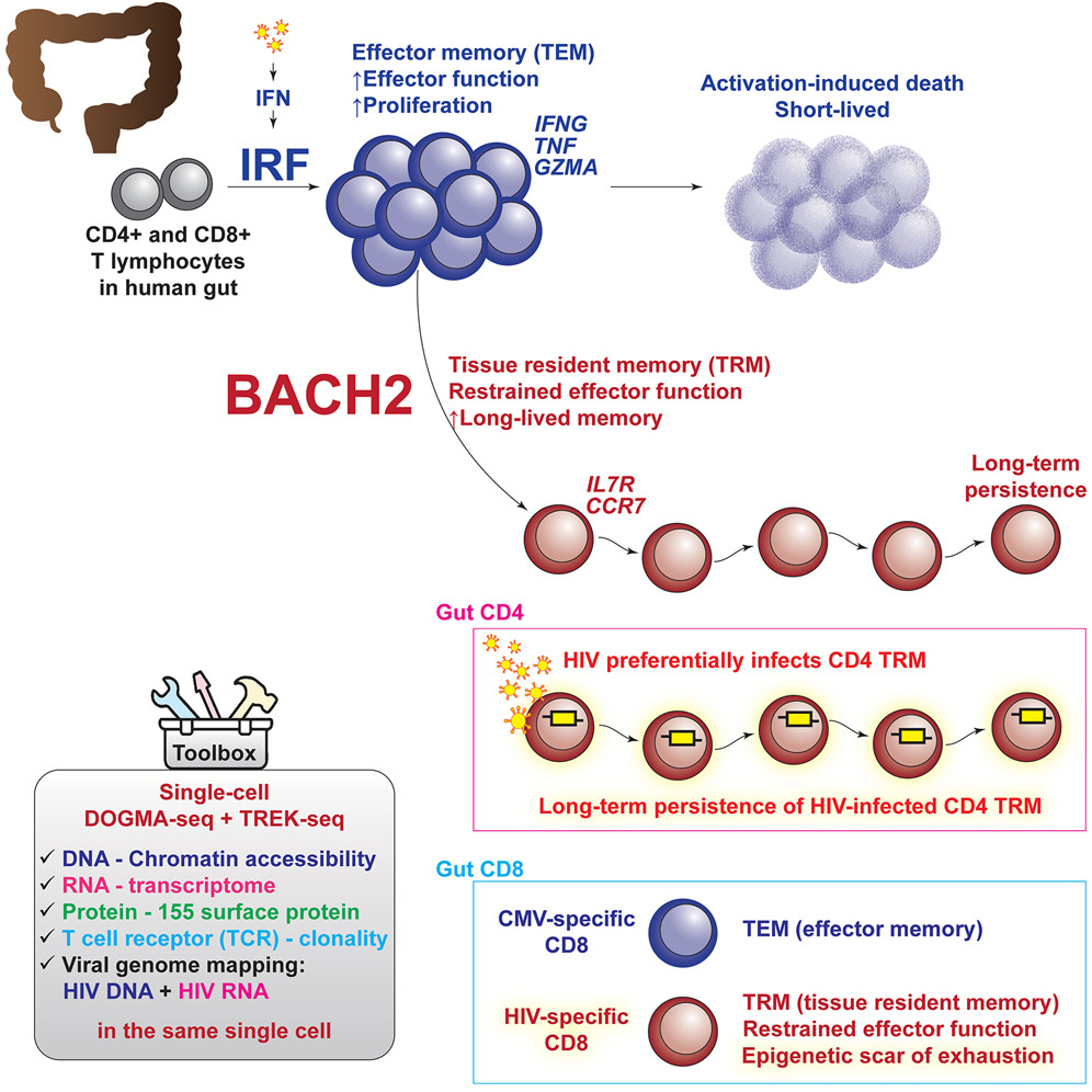
Image source: Wei et al. (2025)
The main focus of this paper was to identify factors involved in HIV persistence within different T-cell populations. In this vein, many of the results were generated after sorting on CD4 and CD8 positive cells to zoom in on those T-cell subtypes. These experiments were also conducted with DOGMA-seq. For the purposes of this workshop we are going to focus on the non-sorted cells, which include immune, epithelial, and glial cell populations.
Samples
This dataset includes 17,642 cells from PLWH and 22,422 cells from HIV-negative individuals. Each PLWH donor was tagged with oligo-barcoded antibodies, pooled, and then sequenced. From all of these cells, the authors were able to identify 16 distinct cell types in the dataset (Figure 2).
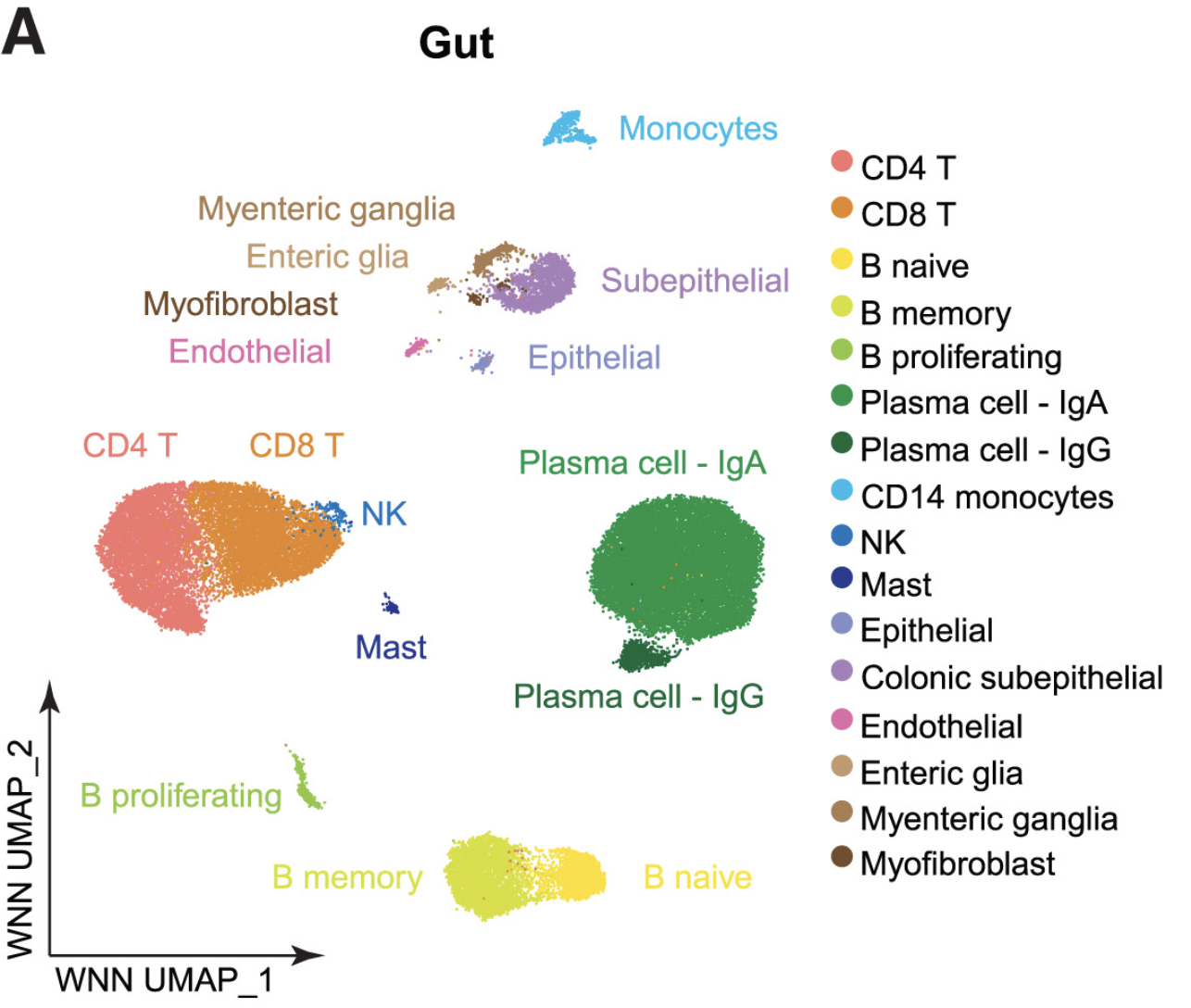
Image source: Wei et al. (2025)
To start, we will be using this heterogeneous population of cells to showcase how multiomics datasets are processed. We will first begin with the hashtags (HTO) and protein expression before moving on to the ATAC-seq material. Lastly, we will pull all three molecular modalities together to run further downstream analyses.
scRNA-seq
Note that we will not discuss the upstream methods used to process scRNA-seq as we have a separate workshop that details those steps in much more depth.
Getting set-up
If you have not already, be sure to download the dataset so that you can access the files used in this analysis. The data can be downloaded from this link.
The dataset is downloaded as a single zipped folder. To get it ready for the workshop:
- Locate the downloaded
.zipfile (usually in yourDownloadsfolder). - Unzip the file by double-clicking on it. This creates a folder called
sc_multiomics. - Move the
sc_multiomicsfolder to yourDesktop, so that it is easy to find throughout the workshop.
Note for Windows OS users
After unzipping, check whether you have a nested sc_multiomics/sc_multiomics folder. If so, move everything from the inner folder up into the outer one, then delete the empty inner folder.
Project organization
When you have large amounts of data, it is easy to lose track of your files and become overwhelmed. We tend to prioritize the analysis and, in the excitement of getting a first look at our data, we often forget to consider how we are going to manage our data and files. This is a common mistake, as data management is often an afterthought when it should be a key part of the workflow from the very beginning. The HMS Data Management Working Group discusses in-depth some aspects to consider beyond the data creation and analysis.
One important aspect of data management is organization. For each experiment you work on and analyze data for, it is considered best practice to get organized by creating a planned storage space. Following these best practices, the files downloaded already follow a structured organization.
Opening RStudio
Inside the sc_multiomics folder on your Desktop, double-click the sc_multiomics.Rproj file. This opens RStudio with the working directory already set to the project folder. The provided file structure should look like Figure 3.
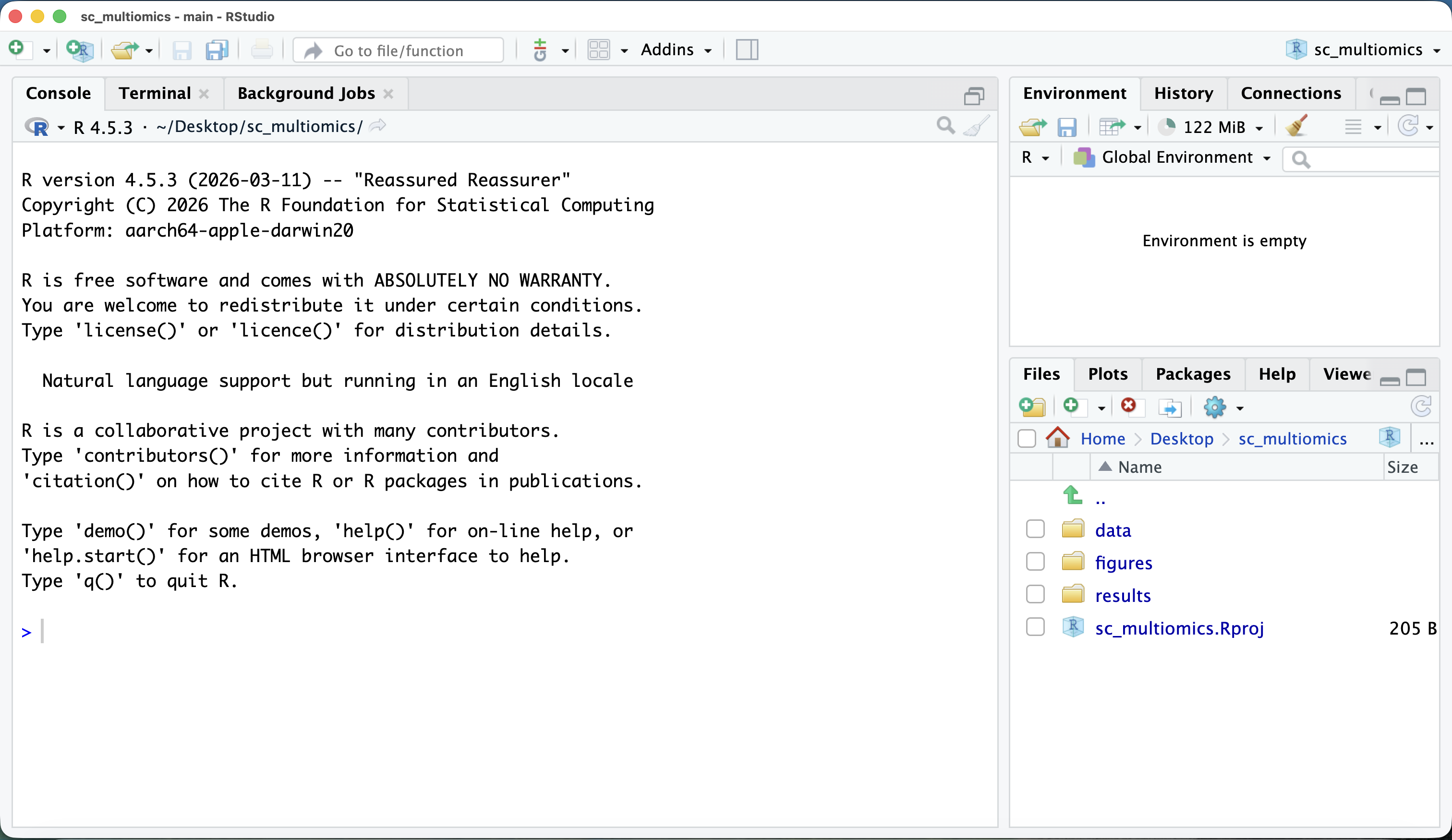
If your RStudio session looks similar to the image above, then you are ready to start!
New script
Next, open a new Rscript file and start with some comments to indicate what this file is going to contain. Ideally, we will have one script per major step in our analysis. For this first script, we will be loading our data, demultiplexing the hashtags (HTO), and processing the protein expression (ADT), as indicated in the header.
Loading your libraries at the top of the script will also allow you to easily keep track of which libraries you are using and to load them all at once in the beginning.
Save the Rscript as 01_demultiplex_hto_and_protein.R in your main folder. Your data directory should look something like this:
data/
├── PT1
│   └── ADT
├── processed_seurat_objects
│   └── seurat_demux.RDS
└── samples.tsv
The data folder contains the raw counts for sample PT1, a processed_seurat_objects folder, and the samples.tsv metadata file. To orient ourselves on how to work with this dataset, we will start by working with the sample PT1.
Sample metadata
A great way to keep track of your samples is to create a samples table that contains all the relevant metadata. Collating all of this information into one spreadsheet will make it easier to match our dataset with the correct experimental conditions.
Inside the data/ folder, we have provided one such metadata file called samples.tsv. For each library, it records the HIV status, the donor(s) it came from, and donor information such as sex, age, race, and treatment. We will first load this in to familiarize ourselves with the data we will be using in the next step.
# Load sample metadata
df_meta <- read_tsv("data/samples.tsv")
df_meta| library | geo_title | hiv_status | patient | donors | sex | age | race | ethnicity | tissue | treatment | collection_date | biosample |
|---|---|---|---|---|---|---|---|---|---|---|---|---|
| B351A | HD351_A_whole | HIV_neg | 351 | 351 | male | 37 | White | Not Hispanic or Latino | colon | none | 2023-10-30 | SAMN48920097 |
| B351B | HD351_B_whole | HIV_neg | 351 | 351 | male | 37 | White | Not Hispanic or Latino | colon | none | 2023-10-30 | SAMN48920097 |
| B351C | HD351_C_whole | HIV_neg | 351 | 351 | male | 37 | White | Not Hispanic or Latino | colon | none | 2023-10-30 | SAMN48920097 |
| B357A | HD357_A_whole | HIV_neg | 357 | 357 | male | 51 | Black | Not Hispanic or Latino | colon | none | 2023-10-30 | SAMN48920098 |
| B357B | HD357_B_whole | HIV_neg | 357 | 357 | male | 51 | Black | Not Hispanic or Latino | colon | none | 2023-10-30 | SAMN48920098 |
| B357C | HD357_C_whole | HIV_neg | 357 | 357 | male | 51 | Black | Not Hispanic or Latino | colon | none | 2023-10-30 | SAMN48920098 |
| B360A | HD360_A_whole | HIV_neg | 360 | 360 | male | 38 | Asian | Not Hispanic or Latino | colon | none | 2023-10-30 | SAMN48920099 |
| B360B | HD360_B_whole | HIV_neg | 360 | 360 | male | 38 | Asian | Not Hispanic or Latino | colon | none | 2023-10-30 | SAMN48920099 |
| B360C | HD360_C_whole | HIV_neg | 360 | 360 | male | 38 | Asian | Not Hispanic or Latino | colon | none | 2023-10-30 | SAMN48920099 |
| B363A | HD363_A_whole | HIV_neg | 363 | 363 | female | 25 | White | Not Hispanic or Latino | colon | none | 2023-10-30 | SAMN48920101 |
| B363B | HD363_B_whole | HIV_neg | 363 | 363 | female | 25 | White | Not Hispanic or Latino | colon | none | 2023-10-30 | SAMN48920101 |
| B363C | HD363_C_whole | HIV_neg | 363 | 363 | female | 25 | White | Not Hispanic or Latino | colon | none | 2023-10-30 | SAMN48920101 |
| PT1 | 035_037_040_pooled_whole | PLWH | pooled | 035;037;040 | male | 37;32;41 | NA;Black;White | Hispanic;Not Hispanic or Latino;Not Hispanic or Latino | colon | Antiretroviral therapy | 2016-08-01;2016-09-21;2016-10-24 | SAMN48920102 |
| PT2 | 008_012_015_pooled_whole | PLWH | pooled | 008;012;015 | male;female;male | 48;47;58 | White;Black;White | Not Hispanic or Latino | colon | Antiretroviral therapy | 2015-08-07;2016-01-20;2016-02-23 | SAMN48920103 |
| PT3 | 017_023_027_029_pooled_whole | PLWH | pooled | 017;023;027;029 | male | 49;45;41;28 | Black;Black;White;Black | Not Hispanic or Latino | colon | Antiretroviral therapy | 2016-04-13;2016-02-15;2016-09-19;2016-05-17 | SAMN48920104 |
| PT4 | 361_pooled_whole | HIV_neg | 361 | 361 | female | 27 | White | Not Hispanic or Latino | colon | none | 2023-07-08 | SAMN48920105 |
This table is valuable because it gives us some key information about each sample. For example, we can see that we have multiple libraries from the same patient for many of the HIV-negative samples. More consequentially, in the patient column, we see the label pooled for all of the PLWH samples. Note that PT4 is a non-pooled HIV-negative sample despite following a different naming convention.
Recall earlier that we discussed that some samples were first tagged with an antibody and then pooled into a single library. This is a common cost-saving technique used to sequence multiple samples at once. However, in doing so, we must computationally determine which cell comes from which sample by using those hash sequences. This process is called demultiplexing which we will discuss more deeply in the next lesson.
Reuse
CC-BY-4.0