Seurat Cheatsheet
This cheatsheet is meant to provide examples of the various functions available in Seurat. This includes how to access certain information, handy tips, and visualization functions built into the package. We have pulled together all of this information with examples using the dataset used throughout this workshop so that there are clear visuals on what the output of each function is.
These materials were developed by referencing the following pages from the Seurat website:
- https://satijalab.org/seurat/articles/essential_commands.html
- https://satijalab.org/seurat/articles/visualization_vignette.html
Dataset
Load in the integrated_seurat object that is available in the data folder of the project. The link to download the project was provided on the schedule page but can also be found here.
library(Seurat)
library(tidyverse)

load(bzfile("data/additional_data/seurat_integrated.RData.bz2"))
seurat_integrated
## An object of class Seurat
## 31130 features across 29629 samples within 3 assays
## Active assay: integrated (3000 features, 3000 variable features)
##  2 layers present: data, scale.data
##  2 other assays present: RNA, SCT
##  2 dimensional reductions calculated: pca, umap
Accessing cell barcodes and gene names
Cell barcodes
Within Seurat, there are multiple ways to access the cell barcode IDs.
We can use colnames() to get a vector of cell barcodes in the same order as they appear in the Seurat object.
colnames(seurat_integrated) %>% head()
## [1] "ctrl_AAACATACAATGCC-1" "ctrl_AAACATACATTTCC-1" "ctrl_AAACATACCAGAAA-1"
## [4] "ctrl_AAACATACCAGCTA-1" "ctrl_AAACATACCATGCA-1" "ctrl_AAACATACCTCGCT-1"
Similarly we can use the Cells() function:
Cells(seurat_integrated) %>% head()
## [1] "ctrl_AAACATACAATGCC-1" "ctrl_AAACATACATTTCC-1" "ctrl_AAACATACCAGAAA-1"
## [4] "ctrl_AAACATACCAGCTA-1" "ctrl_AAACATACCATGCA-1" "ctrl_AAACATACCTCGCT-1"
It is very important that the values stored in Cells() are the same as the rownames in meta.data. Otherwise Seurat will start throwing errors at you!
all(rownames(seurat_integrated@meta.data) == Cells(seurat_integrated))
## [1] TRUE
Features/genes
Now we want to be able to access the rows, or genes, in our Seurat object. Rather than calling these values “genes”, many tools will call them “features” as different assays (CITE-seq, ATAC-seq) provide alternative information than genes as output.
The Features() function returns a vector of all features/genes in our dataset in the same order as it appears in the count matrix.
Features(seurat_integrated) %>% head()
## [1] "FTL" "IGKC" "CCL2" "GNLY" "IGLC2" "CCL3"
The rownames() function provides the same output:
rownames(seurat_integrated) %>% head()
## [1] "FTL" "IGKC" "CCL2" "GNLY" "IGLC2" "CCL3"
Number of cells and features
If you recall, Seurat stores your count matrix as cells (columns) x genes (rows).
Therefore, we can access the number of cells by using the ncol() function.
ncol(seurat_integrated)
## [1] 29629
The number of features is returned with the nrow() function:
nrow(seurat_integrated)
## [1] 3000
The dim() function provides both the number of cells and genes for the default assay. Here we see the number of features followed by the number of cells:
dim(seurat_integrated)
## [1] 3000 29629
Idents
In Seurat, each cell has a label which can be accessed using Idents(). These are the default labels used for each cell and are used internally by Seurat plotting functions.
Common information set as the identity for cells include: clusters (as in our example dataset), celltype, sample, etc. You’ll notice that identities are automatically stored as factors, which means we can re-organize the levels at any point to change their order for plotting purposes.
Idents(seurat_integrated) %>% head()
## ctrl_AAACATACAATGCC-1 ctrl_AAACATACATTTCC-1 ctrl_AAACATACCAGAAA-1
##                     2                     1                     3
## ctrl_AAACATACCAGCTA-1 ctrl_AAACATACCATGCA-1 ctrl_AAACATACCTCGCT-1
##                     3                     4                     1
## Levels: 0 1 2 3 4 5 6 7 8 9 10 11 12 13 14 15 16
Rename Idents
To quickly make modifications to identities, you can use the RenameIdents() function where new values are mapped to the identities. This is particularly helpful when annotating your cells from clusters to celltypes as showcased here. Bear in mind that these new identities are not stored in the meta.data automatically. We recommend adding these identities as a new column in the Seurat object to keep track of it for future use.
# Rename all identities
seurat_integrated <- RenameIdents(object = seurat_integrated,
                                 "0" = "Naive or memory CD4+ T cells",
                                 "1" = "CD14+ monocytes",
                                 "2" = "Activated T cells",
                                 "3" = "CD14+ monocytes",
                                 "4" = "Stressed cells / Unknown",
                                 "5" = "CD8+ T cells",
                                 "6" = "Naive or memory CD4+ T cells",
                                 "7" = "B cells",
                                 "8" = "NK cells",
                                 "9" = "CD8+ T cells",
                                 "10" = "FCGR3A+ monocytes",
                                 "11" = "B cells",
                                 "12" = "NK cells",
                                 "13" = "B cells",
                                 "14" = "Conventional dendritic cells",
                                 "15" = "Megakaryocytes",
				 "16" = "Plasmacytoid dendritic cells")

# These new celltype values are only stored in the idents
# Good practice is to store these changes in a column
seurat_integrated$celltype <- Idents(seurat_integrated)
Highly variable features
Accessing variable features
To obtain a vector of all highly variable genes that were selected after running FindVariableFeatures(), we can use the VariableFeatures() function.
VariableFeatures(seurat_integrated) %>% head()
## [1] "FTL" "IGKC" "CCL2" "GNLY" "IGLC2" "CCL3"
Setting variable features
Using the same VariableFeatures() function, we can set our own custom set of genes as our highly variable genes.
As an example, here we are omitting mitochondrial genes from the original list of variable genes:
# Get list of all variable genes
# Remove variable genes that start with MT-
var_genes <- VariableFeatures(seurat_integrated)
var_genes <- var_genes[!startsWith(var_genes, "MT-")]

# Now we set our vector of gene names back to VariableFeatures()
VariableFeatures(seurat_integrated) <- var_genes
Assays and layers
Assays
Within a Seurat object you can have multiple “assays”. Each assay contains its own count matrix that is separate from the other assays in the object. This structure was created with multimodal datasets in mind so we can store, for example, ATAC peaks within the same Seurat object as your RNA counts.
SCTransform also makes use of these assays to store the SCT normalized matrix in a separate assay called “SCT”.
To access the list of assays in your Seurat object, you can call @assays.
seurat_integrated@assays
## $RNA
## Assay data with 14065 features for 29629 cells
## First 10 features:
##  AL627309.1, AL669831.5, LINC00115, FAM41C, NOC2L, KLHL17, PLEKHN1,
## HES4, ISG15, AGRN
##
## $SCT
## SCTAssay data with 14065 features for 29629 cells, and 2 SCTModel(s)
## First 10 features:
##  AL627309.1, AL669831.5, LINC00115, FAM41C, NOC2L, KLHL17, PLEKHN1,
## HES4, ISG15, AGRN
##
## $integrated
## SCTAssay data with 3000 features for 29629 cells, and 1 SCTModel(s)
## Top 10 variable features:
##  FTL, IGKC, CCL2, GNLY, IGLC2, CCL3, CCL4, CXCL10, CCL7, TIMP1
We can additionally see which of the assays in our dataset is set as the default with the DefaultAssays() function. This default assay is automatically used as by Seurat functions, unless you specify otherise in the parameters of your function.
DefaultAssay(seurat_integrated)
## [1] "integrated"
Here we can see that the default assay is set to “integrated”. If we instead wanted to use the RNA counts, we can set a new default by once again calling the DefaultAssay() function and storing the name of a different assay.
# Set new default assay
DefaultAssay(seurat_integrated) <- "RNA"

# Print out the new default to see if it changed
DefaultAssay(seurat_integrated)
## [1] "RNA"
We can access each assay as if the Seurat object was a named list with double brackets:
seurat_integrated[["SCT"]]
## SCTAssay data with 14065 features for 29629 cells, and 2 SCTModel(s)
## First 10 features:
##  AL627309.1, AL669831.5, LINC00115, FAM41C, NOC2L, KLHL17, PLEKHN1,
## HES4, ISG15, AGRN
And similarly run any function on it:
dim(seurat_integrated[["integrated"]])
## [1] 3000 29629
Layers
Layers are the different counts matrices that you can access within each assay (prior to Seurat version 5, this feature was known as “slots”).
Following the standard Seurat workflow, you would have the following matrices:
- counts (raw counts matrix)
- data (normalized count matrix (generated after
SCTransform()orNormalizeData()) - scale.data (output from the
ScaleData())
We can see which layers are accessible with the Layers() function.
Layers(seurat_integrated[["RNA"]])
## [1] "counts" "data"
In this object we can see that we do not have the scale.data layer currently. So if we run ScaleData() we will be able to access this layer/matrix.
seurat_integrated <- ScaleData(seurat_integrated)
Layers(seurat_integrated)
## Centering and scaling data matrix

## [1] "counts"     "data"       "scale.data"
Accessing full count matrix
You can grab the entire counts matrix by making use of the LayerData() function.
# Subsetting to the first 5 genes and cells for easy viewing
LayerData(seurat_integrated, assay="RNA", layer="counts")[1:5, 1:5]
## 5 x 5 sparse Matrix of class "dgCMatrix"
##            ctrl_AAACATACAATGCC-1 ctrl_AAACATACATTTCC-1 ctrl_AAACATACCAGAAA-1
## AL627309.1                     .                     .                     .
## AL669831.5                     .                     .                     .
## LINC00115                      .                     .                     .
## FAM41C                         .                     .                     .
## NOC2L                          .                     .                     .
##            ctrl_AAACATACCAGCTA-1 ctrl_AAACATACCATGCA-1
## AL627309.1                     .                     .
## AL669831.5                     .                     .
## LINC00115                      .                     .
## FAM41C                         .                     .
## NOC2L                          .                     .
Accessing specific features and metadata
The FetchData() function is useful to directly access the counts of a feature for each cell. You can also specify the layer and assay to specify which piece of information you want.
# Normalized counts for the gene PTPRC in the assay SCT
FetchData(seurat_integrated, vars=c("PTPRC", "sample"), assay="SCT", layer="data") %>% head()
##                          PTPRC sample
## ctrl_AAACATACAATGCC-1 2.254699   ctrl
## ctrl_AAACATACATTTCC-1 1.435328   ctrl
## ctrl_AAACATACCAGAAA-1 1.584935   ctrl
## ctrl_AAACATACCAGCTA-1 1.403025   ctrl
## ctrl_AAACATACCATGCA-1 2.667563   ctrl
## ctrl_AAACATACCTCGCT-1 0.000000   ctrl
Conveniently, you can also get information from multiple assays at the same time. To do so, you prepend the assay name (in lowercase format) for the feature you supply to the FetchData() function.
# Grab the normalized counts in the integrated and RNA assays
FetchData(seurat_integrated, vars=c("rna_PTPRC", "integrated_PTPRC"), layer="data") %>% head()
##                       rna_PTPRC integrated_PTPRC
## ctrl_AAACATACAATGCC-1  2.254699        0.4585611
## ctrl_AAACATACATTTCC-1  1.435328       -0.3528445
## ctrl_AAACATACCAGAAA-1  1.584935       -0.1980966
## ctrl_AAACATACCAGCTA-1  1.403025       -0.3175056
## ctrl_AAACATACCATGCA-1  2.667563        0.7853486
## ctrl_AAACATACCTCGCT-1  0.000000       -0.8399404
Accessing dimensional reductions
PCA
The scores for each PC is stored within the embeddings slot of the Seurat object. These can be accessed by using the Embeddings() function.
# Alternative method of accessing PCA values
# seurat_integrated[['pca']]@cell.embeddings

Embeddings(seurat_integrated, reduction="pca")[1:5, 1:5]
##                              PC_1      PC_2      PC_3       PC_4        PC_5
## ctrl_AAACATACAATGCC-1 -14.9778236 -2.879193 -5.059351  -1.602766   0.8728779
## ctrl_AAACATACATTTCC-1  22.3923271 -5.296913  4.951958   3.112632   0.3379874
## ctrl_AAACATACCAGAAA-1  28.9847264  1.203408 -5.947993  -1.042701  -7.5690434
## ctrl_AAACATACCAGCTA-1  20.1284164  2.826128 -5.265061  -3.620790 -11.3740400
## ctrl_AAACATACCATGCA-1  -0.4713399  1.122713  5.195209 -23.884004  -2.2996247
The weight (loadings) for each feature is also stored and can be accessed with Loadings() function.
# pbmc[['pca]]@feature.loadings
Loadings(seurat_integrated, reduction="pca")[1:5, 1:5]
##               PC_1         PC_2        PC_3        PC_4        PC_5
## FTL    0.424580221 -0.029245940 -0.07877921 -0.01084091 -0.17392237
## IGKC  -0.022397858 -0.113342789  0.24606406  0.09924655 -0.08598287
## CCL2   0.138755172  0.002935082 -0.07471508 -0.02671091 -0.25223145
## GNLY  -0.017962104  0.357256939  0.07523939  0.10126832 -0.05577892
## IGLC2 -0.007534059 -0.037760970  0.07610433  0.03463625 -0.02070632
We can also view more information about the top PCs, like the genes that are most strongly correlated with the first few PCs with the ProjectDim() function.
ProjectDim(seurat_integrated, reduction = "pca")
## PC_ 1
## Positive:  FTL, TIMP1, FTH1, C15orf48, CXCL8, CCL2, S100A8, FCER1G, TYROBP, S100A4
##     CD63, LGALS3, LYZ, S100A9, ACTB, LGALS1, ANXA5, HLA-DRA, SOD2, S100A11
## Negative:  RPL3, RPL13, RPS6, RPS18, RPL10, RPL21, RPL13A, RPS2, RPS4X, RPS3
##     RPS14, RPL32, RPL7, PABPC1, RPS19, RPL34, TRAC, RPS3A, RPS27A, TRBC1
## PC_ 2
## Positive:  GNLY, CCL5, NKG7, GZMB, FGFBP2, CST7, APOBEC3G, GZMH, KLRD1, CLIC3
##     PRF1, GZMA, CTSW, CHST12, HOPX, HLA-A, CCL4, RARRES3, HLA-B, AOAH
## Negative:  CD74, IGHM, IGKC, HLA-DRA, CD79A, CCR7, RPL13, HLA-DRB1, EEF1A1, RPS18
##     RPS6, RPL10, RPL32, PABPC1, RPL18A, RPS2, LTB, HLA-DQA1, HLA-DQB1, RPL13A
## PC_ 3
## Positive:  CD74, IGKC, HLA-DRA, IGHM, HLA-DRB1, HLA-DQA1, HLA-DPA1, CD79A, HLA-DPB1, HLA-DQB1
##     CD83, HERPUD1, MS4A1, ID3, HLA-DMA, IGLC2, GNLY, HSP90AB1, CD79B, GZMB
## Negative:  TRAC, FTL, CCL2, PABPC1, S100A8, TRBC1, CD3D, GIMAP7, RPS18, RPS14
##     RPL3, RPL13, S100A9, FTH1, RPL34, RPL10, RPS4X, LTB, SARAF, RPL21
## PC_ 4
## Positive:  CD74, IGHM, CCL5, GNLY, IGKC, NKG7, HLA-DRA, GZMB, RPL3, CD79A
##     HLA-DPB1, RPL10, RPS2, HLA-DPA1, HLA-DRB1, RPS4X, RPL13, EEF1A1, RPS18, RPS19
## Negative:  HSPB1, CACYBP, HSPH1, HSP90AB1, HSPA8, SRSF7, SRSF2, UBC, HSPA1A, UBB
##     YPEL5, H3F3B, DNAJB6, GADD45B, HSPE1, EIF1, DDIT4, RSRC2, ZFAND2A, DNAJB1
## PC_ 5
## Positive:  VMO1, FCGR3A, MS4A7, TIMP1, TNFSF10, CXCL10, CALHM6, CXCL16, MS4A4A, LST1
##     JPT1, AIF1, IFITM3, GBP1, SAT1, ATP1B3, GBP5, TNFSF13B, FGL2, PLAC8
## Negative:  CCL2, FTL, CXCL8, S100A8, S100A9, CCL7, CXCL3, IGKC, IGHM, CTSL
##     CD63, CXCL2, LGALS3, PLA2G7, CSTB, IL1B, CXCL1, SERPINB2, CTSB, GNLY
UMAP/tSNE
To access the coordinates used for UMAP/tSNE plots, we specify the reduction of interest in the Embeddings() function.
# seurat_integrated[['umap']]@cell.embeddings
Embeddings(seurat_integrated, reduction="umap") %>% head()
##                           UMAP_1     UMAP_2
## ctrl_AAACATACAATGCC-1   7.270473  0.9072988
## ctrl_AAACATACATTTCC-1  -8.742020  1.5622634
## ctrl_AAACATACCAGAAA-1 -10.032904  4.7139827
## ctrl_AAACATACCAGCTA-1  -8.363044  5.0377137
## ctrl_AAACATACCATGCA-1   6.875784 -4.6442526
## ctrl_AAACATACCTCGCT-1  -9.338899  2.2808882
Data visualization
Underneath the hood, all of Seurat’s plotting functions make use of ggplot which means that we can add more details to our plots using ggplot functions.
DimPlot
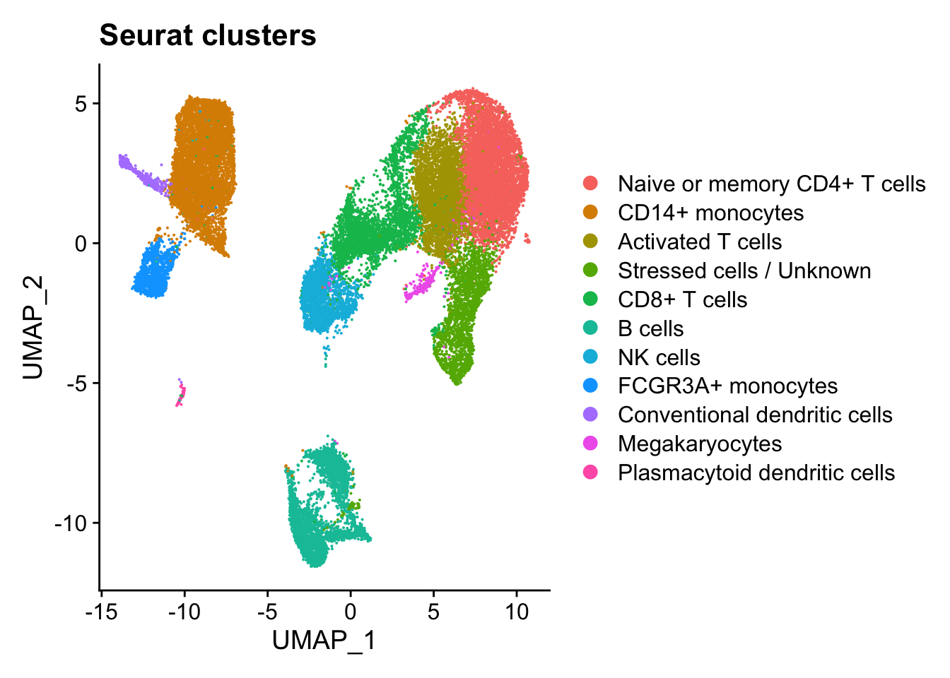
The DimPlot() function allows us to visualize metadata that is categorical on different reductions (PCA, UMAP).
By default DimPlot() will color cells by the Idents() and use UMAP as the default reduction.
DimPlot(seurat_integrated) + ggtitle("Seurat clusters")
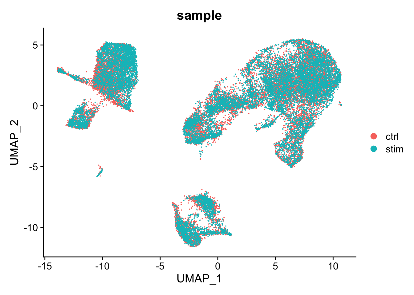
We can specify a different metadata column using the group.by argument
DimPlot(seurat_integrated, group.by = "sample")
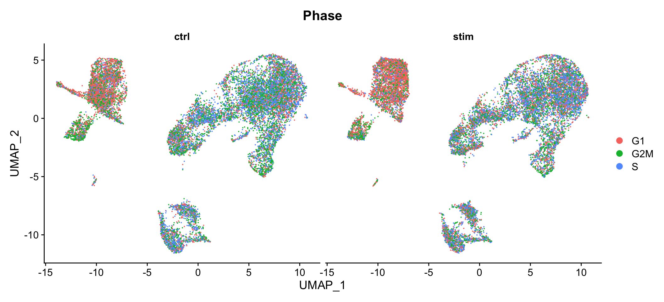
We can also use the split.by argument to create multiple plots that only show cells that have the same value for the metadata column specified.
DimPlot(seurat_integrated, split.by = "sample", group.by="Phase")
FeaturePlot
The FeaturePlot() function allows us to visualize both metadata and features that are continuous on different reductions (PCA, UMAP).
FeaturePlot(seurat_integrated, features = c("FCGR3A", "MS4A7"))
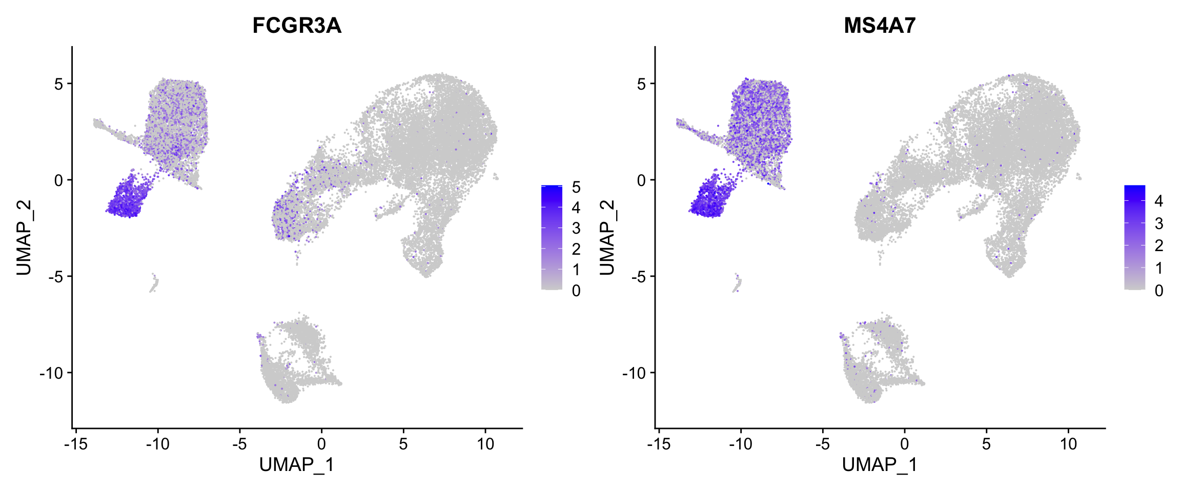
We can additionally order the values in a way that cells with higher values are shown in front (to avoid other cells drowning out them).
To identify cells that show the highest expression of a feature, we can set a min.cutoff based upon quantiles, where cells below the the threshold will show no expression.
FeaturePlot(seurat_integrated,
            reduction = "umap",
            features = c("FCGR3A", "MS4A7"),
            order = TRUE,
            min.cutoff = 'q10')

We can also add labels onto our UMAP to easily identify which groups of cells we are seeing the expression using the LabelClusters() function. The parameters shown here put a white background behind the text to make it easier to see the labels.
Idents(seurat_integrated) <- "integrated_snn_res.0.8"
p <- FeaturePlot(seurat_integrated,
            reduction = "umap",
            features = "FCGR3A",
            order = TRUE,
            min.cutoff = 'q10')
LabelClusters(p, id = "ident",  fontface = "bold", size = 3, bg.colour = "white", bg.r = .2, force = 0)

FeatureScatter
FeatureScatter() creates a scatterplot of expression values for two features with each cell being colored by the ident. Bear in mind that you can also specify a continuous metadata column and not just 2 genes/features.
Idents(seurat_integrated) <- "celltype"
FeatureScatter(seurat_integrated, feature1 = "MT-ND5", feature2 = "mitoRatio") + ggtitle("MitoRatio vs MT-ND5 expression")

CellScatter
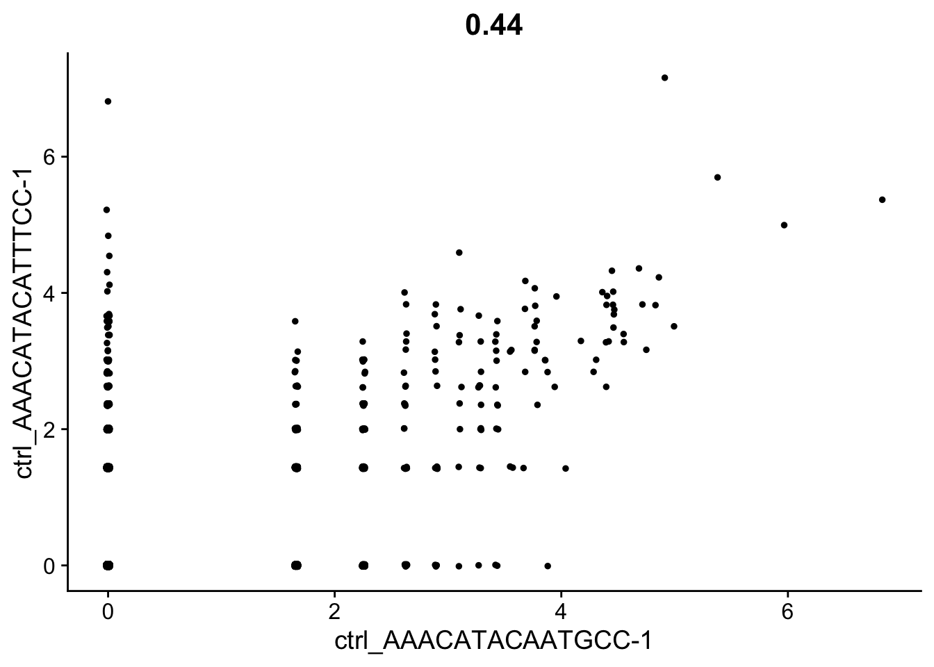
To visualize the differences between two specific cells, you can use the CellScatter() function to get a scatterplot of values for each feature in both cells.
cell1 <- Cells(seurat_integrated)[1]
cell2 <- Cells(seurat_integrated)[2]

# Here we can see the metadata for the first two cells in the dataset
# We are comparing "Activated T cell" vs "CD14+ monocytes" (so they should be very different)
seurat_integrated@meta.data %>% subset(cells %in% c(cell1, cell2)) %>% select(sample, celltype)
CellScatter(seurat_integrated, cell1=cell1, cell2=cell2)
VlnPlot
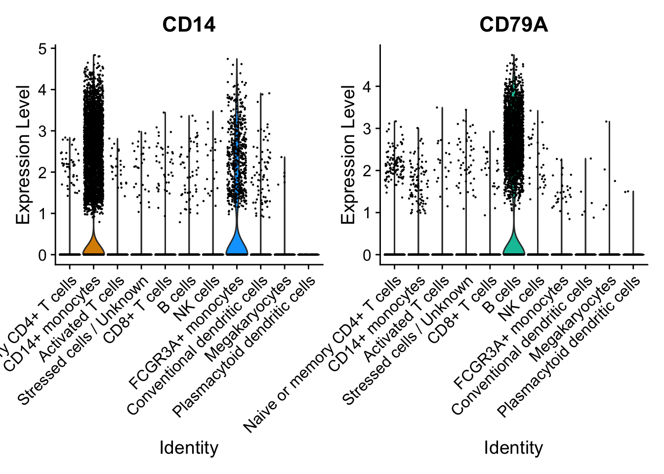
We can create a violin plot to compare the distribution of gene expression across different populations using the VlnPlot() function.
This is a very customizable function, with many parameters to customize the look of the plots.
VlnPlot(seurat_integrated, c("CD14", "CD79A"))
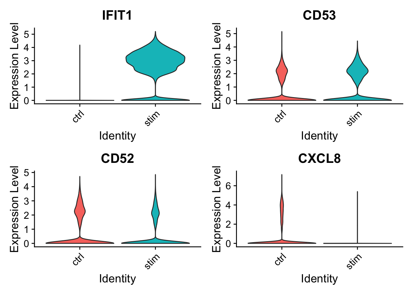
In this example, we are grouping expression by sample and showing 2 plots per column. We are also removing the points (cells) by setting their size to 0.
VlnPlot(seurat_integrated, c("IFIT1", "CD53", "CD52", "CXCL8"), group.by="sample", ncol=2, pt.size=0)
RidgePlot
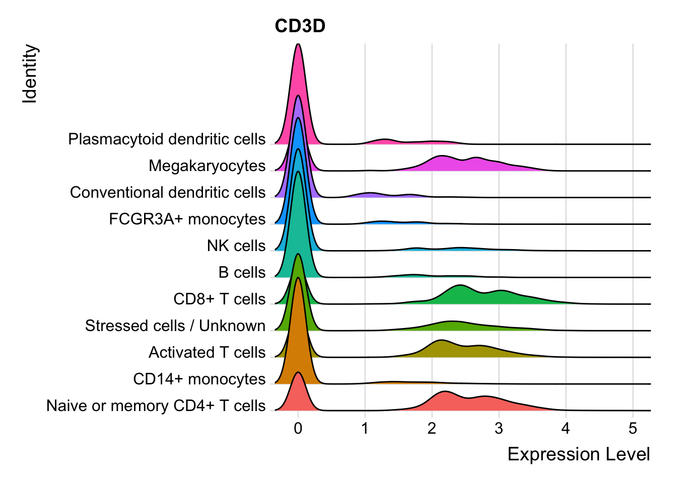
Ridge plots are most commonly used with CITE-seq or hashtagged dataset as they provide an easy way to identify cells that express a protein/antibody.
For our scRNA dataset, when we call RidgePlot(), on the y-axis we see the unique identities assigned for each cell. The x-axis shows us the expression level for whichever feature we chose. This is a great visualization to use when justifying annotation decisions.
RidgePlot(seurat_integrated, "CD3D", assay="RNA") + NoLegend()
DimHeatmap
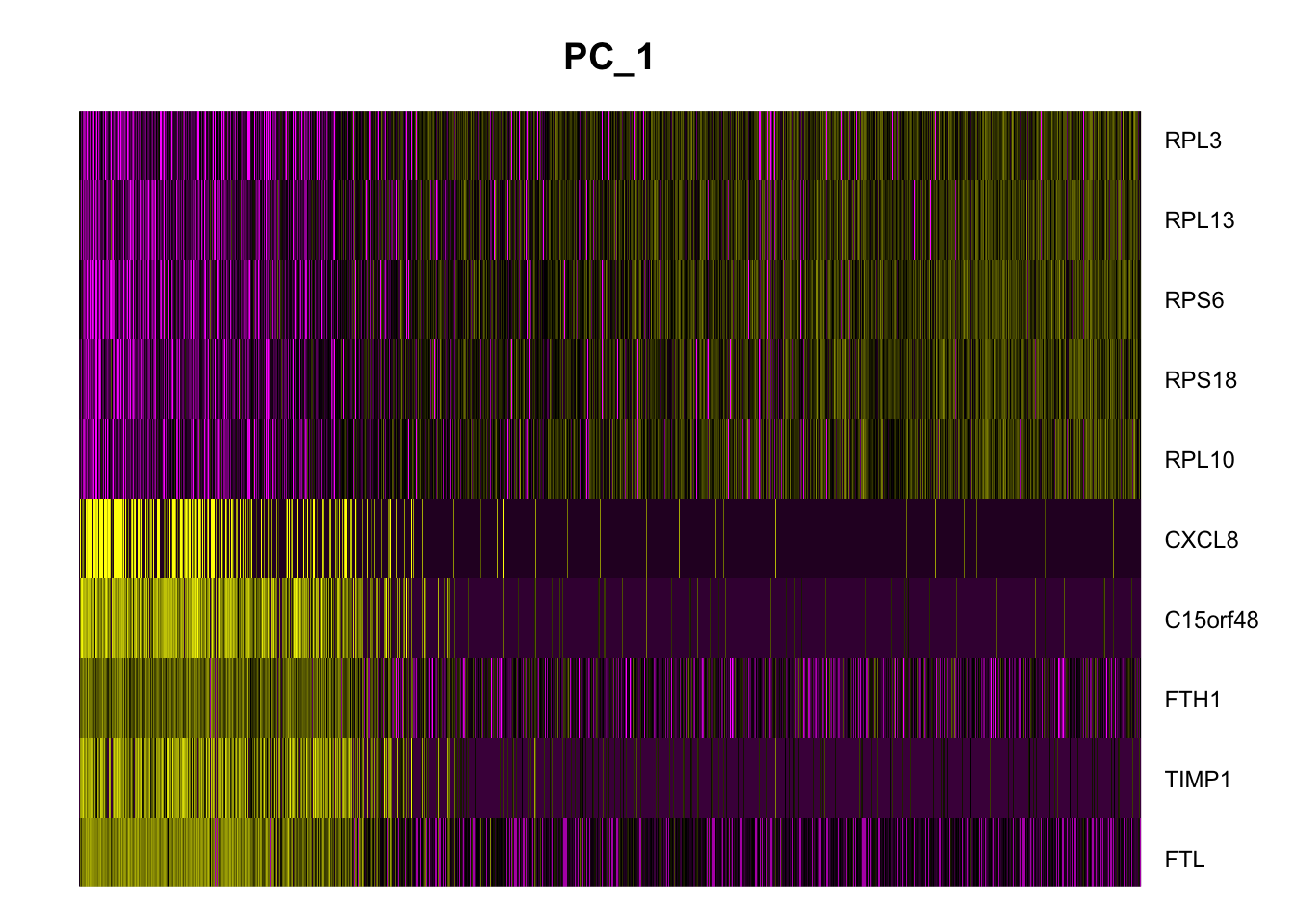
To see the effect of genes on the principal component, we can see the top and bottom features in PC1 using the DimHeatmap() function.
DimHeatmap(seurat_integrated, nfeatures = 10)
DoHeatmap
To plot the expression values for genes across all cells (grouped by their identity), you can call Seurat’s DoHeatmap() function to identify which populations certain genes are lowly or hihgly expressed.
Idents(seurat_integrated) <- "celltype"
DoHeatmap(seurat_integrated, features=c("CD14", "FCGR3A", "FCER1A", "IL3RA", "CD79A", "CD3D"))

DotPlot
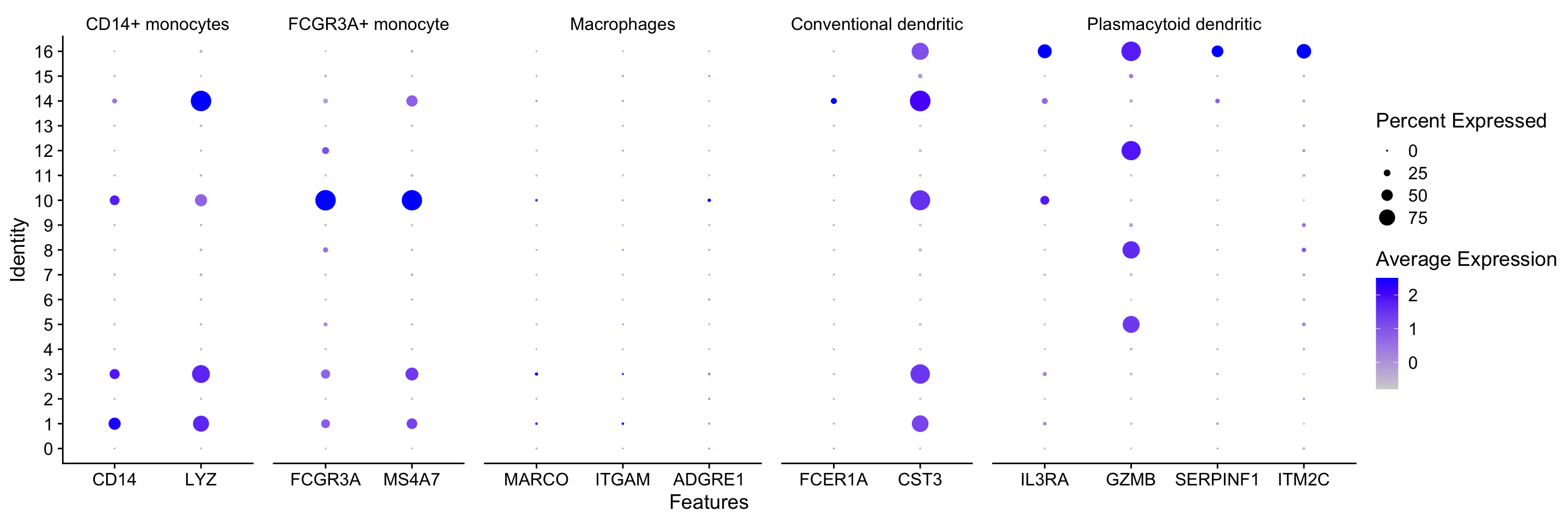
Seurat also has a built in visualization tool which allows us to view the average expression of genes groups clusters called DotPlot(). The size of the circle represents the number of cells that express the gene within a group and the hue reprents the average expression of the feature.
If you supply a named list with labels annotating genes, those labels will appear at the top of the plot for easier visualization.
# List of known celltype markers
markers <- list()
markers[["CD14+ monocytes"]] <- c("CD14", "LYZ")
markers[["FCGR3A+ monocyte"]] <- c("FCGR3A", "MS4A7")
markers[["Macrophages"]] <- c("MARCO", "ITGAM", "ADGRE1")
markers[["Conventional dendritic"]] <- c("FCER1A", "CST3")
markers[["Plasmacytoid dendritic"]] <- c("IL3RA", "GZMB", "SERPINF1", "ITM2C")

# Create dotplot based on RNA expression
DotPlot(seurat_integrated, markers, assay="RNA", group.by = "integrated_snn_res.0.8")
