Contributors: Heather Wick, Upendra Bhattarai, Meeta Mistry, Will Gammerdinger
Approximate time:
Learning objectives
- Visualize peaks in IGV (Integrative Genomics Viewer)
- Qualitatively assess whether DiffBind correctly identifies differential binding
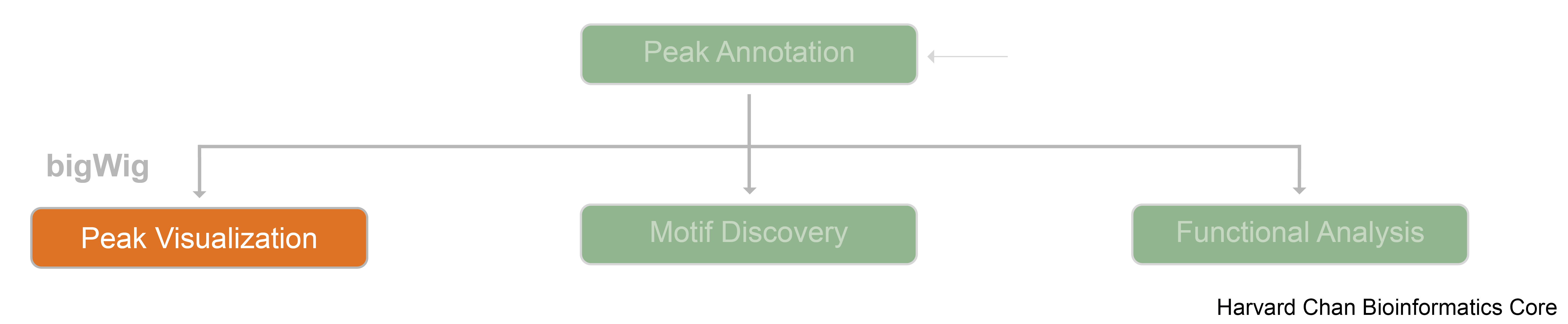
Overview
![]()
When working with next-generation sequecing data, it can be helpful to visualize your analysis. Integrative Genomics Viewer (IGV) is an open-source desktop genome visualization tool that supports visualization for a wide variety of file formats including:
- BED
- bigWig
- VCF
- BAM/SAM
- wig
- bedGraph
- narrowPeak/broadPeak
- GFF3
- GTF
- More and with a complete list of suppported file formats can be found here
Below we will learn about the file formats used to visualize peaks in IGV and use it to explore peaks in our experiment samples.
IGV
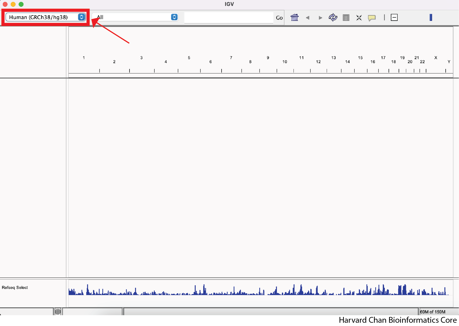
Select the mm10 reference genome
Open IGV on your computer. The first thing we will need to do is select the appropriate reference genome (mm10). There should be a dropdown menu in the top left of IGV, which lets you select your preferred reference genome. If your selected reference genome is already mm10, then you can skip the next few steps. Otherwise, left-click on the dropdown menu:
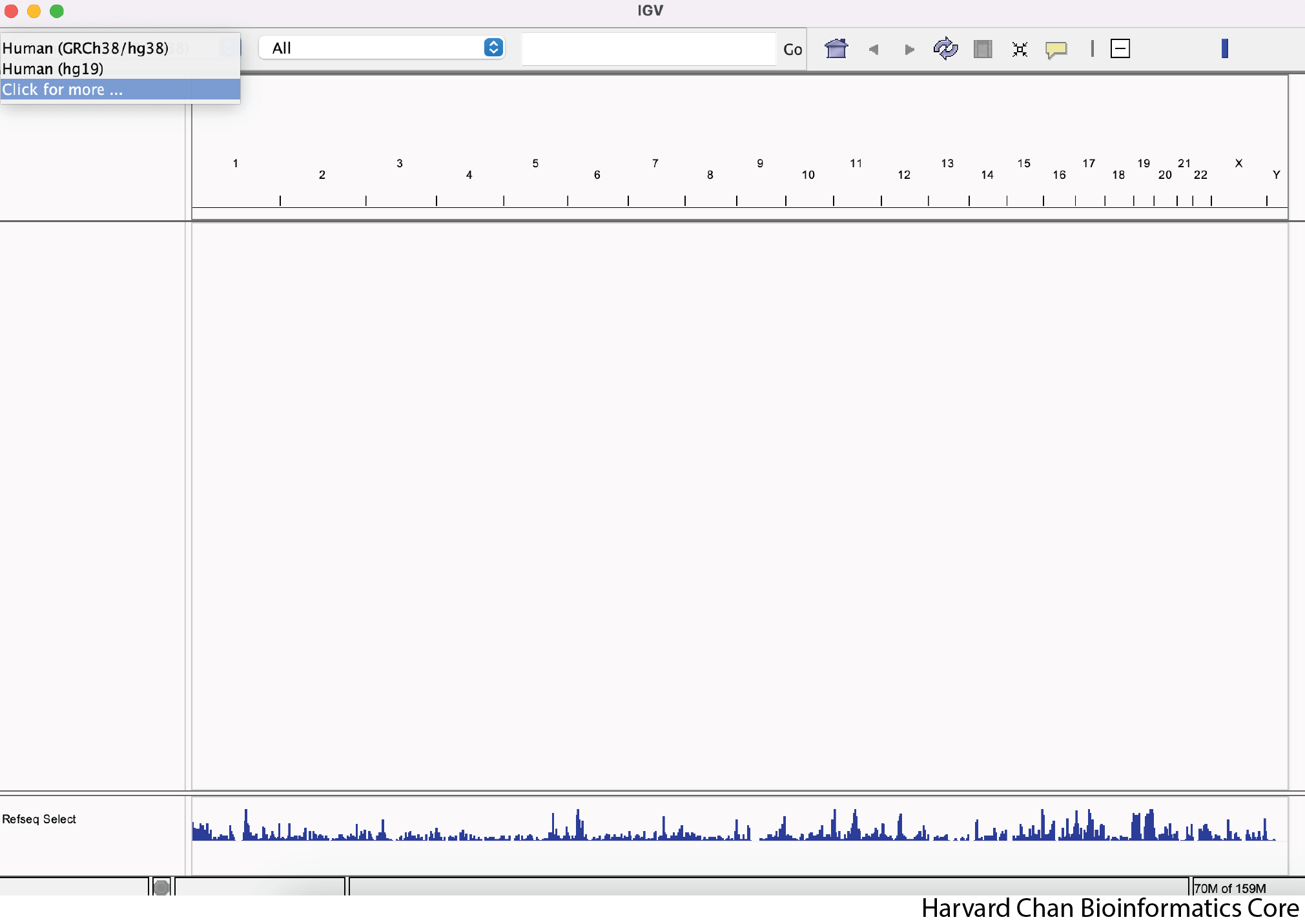
You can see a few options for reference genomes to select from. If you see mm10, then you can select it. Otherwise, left-click on “Click for more …”
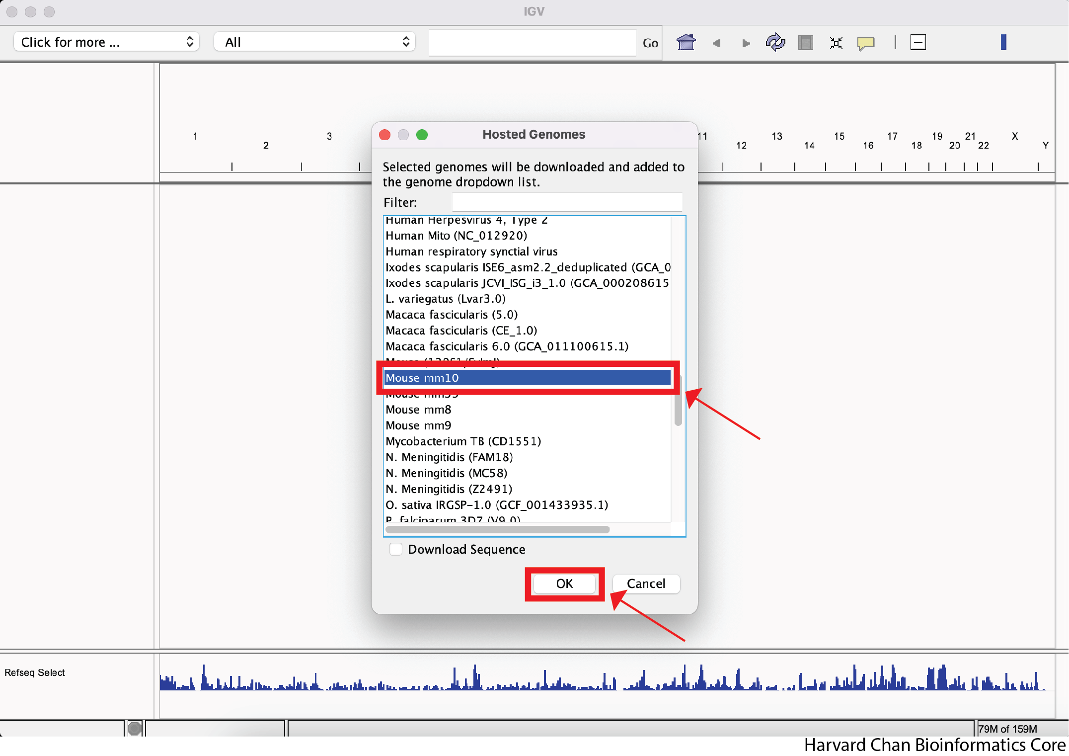
Find “Mouse mm10” from the menu and left-click “OK”.
Download files for visualization
Next, we need to download some files that we will be visualizing in IGV. Right-click this link and select “Save Link As…” to download the ZIP compressed directory of the BigWig files from Dropbox. Place this file within the data folder of your Peak_analysis. Repeat this process with this link for the BED file of differentially called peaks from DiffBind and also place this file within the data folder of your Peak_analysis.
Click here to see how to create bigWig files
We will need to use the output from thepicard`'s CollectAlignmentSummaryMetrics tool once again. As a reminder the code for running this would be:# Run picard CollectAlignmentSummaryMetrics for a sample java -jar picard.jar CollectAlignmentSummaryMetrics \ --INPUT $INPUT_BAM \ --REFERENCE_SEQUENCE $REFERENCE \ --OUTPUT $OUTPUT_METRICS_FILE
We will be interested in the value associated with
PF_READS_ALIGNED. This is the number of your mapped reads. We will use this number to create a scaling factor in the next step to create a bedGraph file.The full documentation for
picard CollectAlignmentSummaryMetrics can be found here.In order to create a bedGraph file we will use
bedtools's genomecov tool.
$SCALE_FACTOR=`awk 'BEGIN { print 1000000 / $MAPPED_READ_COUNT }'`

bedtools genomecov \
  -ibam $INPUT_SORTED_BAM \
  -bg \
  -scale $SCALE_FACTOR | \
  sort -k1,1 -k2,2n \
  > $OUTPUT_FILE
We will need to create a bash variable to hold a scale factor to a million, which we will call in the
bedtools command. The command to do this is:$SCALE_FACTOR=`awk 'BEGIN { print 1000000 / $MAPPED_READ_COUNT }'`bedtools genomecov- Calls thebedtools'sgenomecovtool-ibam- Input sorted BAM file-bg- Output depth in bedGraph format-scale- Scale factor used for scaling the datasort -k1,1 -k2,2n- The output file is unsorted and needs to be sorted by chromosome and chromosome start location> $OUTPUT_FILE- Write to an output file
The full documentation for
bedtools genomecov can be found here.
At this point it is possible to load bedGraph formatted files into IGV, but they are much larger than BigWig files, so we will convert our bedGraph files into BigWig files using a tool called bedGraphToBigWig:
bedGraphToBigWig \
    $BEDGRAPH_INPUT \
    $CHROMOSOME_SIZES_FILE \
    $BIGWIG_OUTPUT
We can break this command down as:
bedGraphToBigWig- Calls thebedGraphToBigWigtool$BEDGRAPH_INPUT- The bedGraph input file$CHROMOSOME_SIZES_FILE- A tab-delimited file with chromosomes in the first column and their associated sizes in the second column. For more information on how to create this file, click on the dropdown below called "Click here to see how to create a chromosome sizes file"$BIGWIG_OUTPUT- The BigWig output file
The download for
bedGraphToBigWig can be found here.Click here to see how to create a chromosome sizes file
There are several ways to make a tab-delimited file with the chromosomes in the first column and their associated sizes in the second column. One way is to use thesamtools package faidx to create a FASTA index file. The documentation to run this cool can be found here. The command to run the samtools faidx tool is:
  samtools faidx \
    $REFERENCE_GENOME_FASTA
We can break this command into two parts:
samtools faidx- Call thesamtools faidxtool$REFERENCE_GENOME_FASTA- The reference genome FASTA file
The full documentation for using
samtools faidx can be found here.However, this output will have a few more columns than you need. You only need the first two columns, so we can use
awk to parse out the first two columns:
  awk \
  -v OFS='\t' \
  '{print $1, $2}' \
  $FASTA_INDEX_FILE \
  > $CHROMOSOME_SIZES_FILE
This command is composed of a few parts:
awk- Callingawk-v OFS='\t'- Output as tab-delimited'{print $1, $2}'- Print the first and second columns$FASTA_INDEX_FILE- Input FASTA index file that was made with the abovesamtools faidxcommand> $CHROMOSOME_SIZES_FILE- Output chromosome sizes file that we can use in ourbedGraphToBigWigcommand
Loading Tracks
Loading Tracks from Files
Now that we have the data that we would like to visualize, let’s go ahead and load it into IGV. Many file formats you load into IGV will load as a single “track”, or horizontal row of genomic data. However, some, like BAM/SAM, will load as multiple tracks. Let’s go ahead and load the BigWig track for our cKO IP replicate 3 sample.
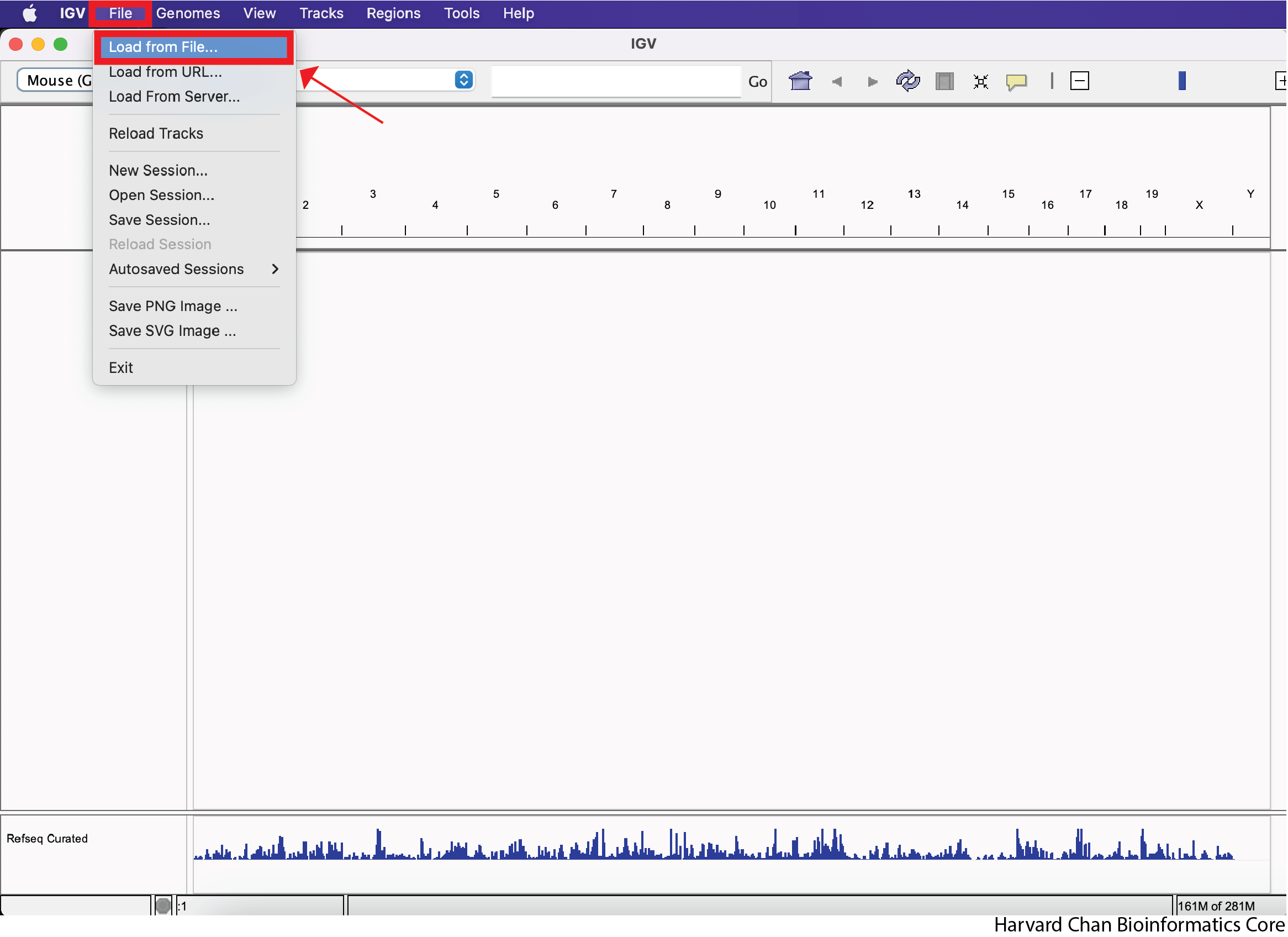
In order to load a track from a file, left-click on “File” in the top-left and select “Load from File…”:
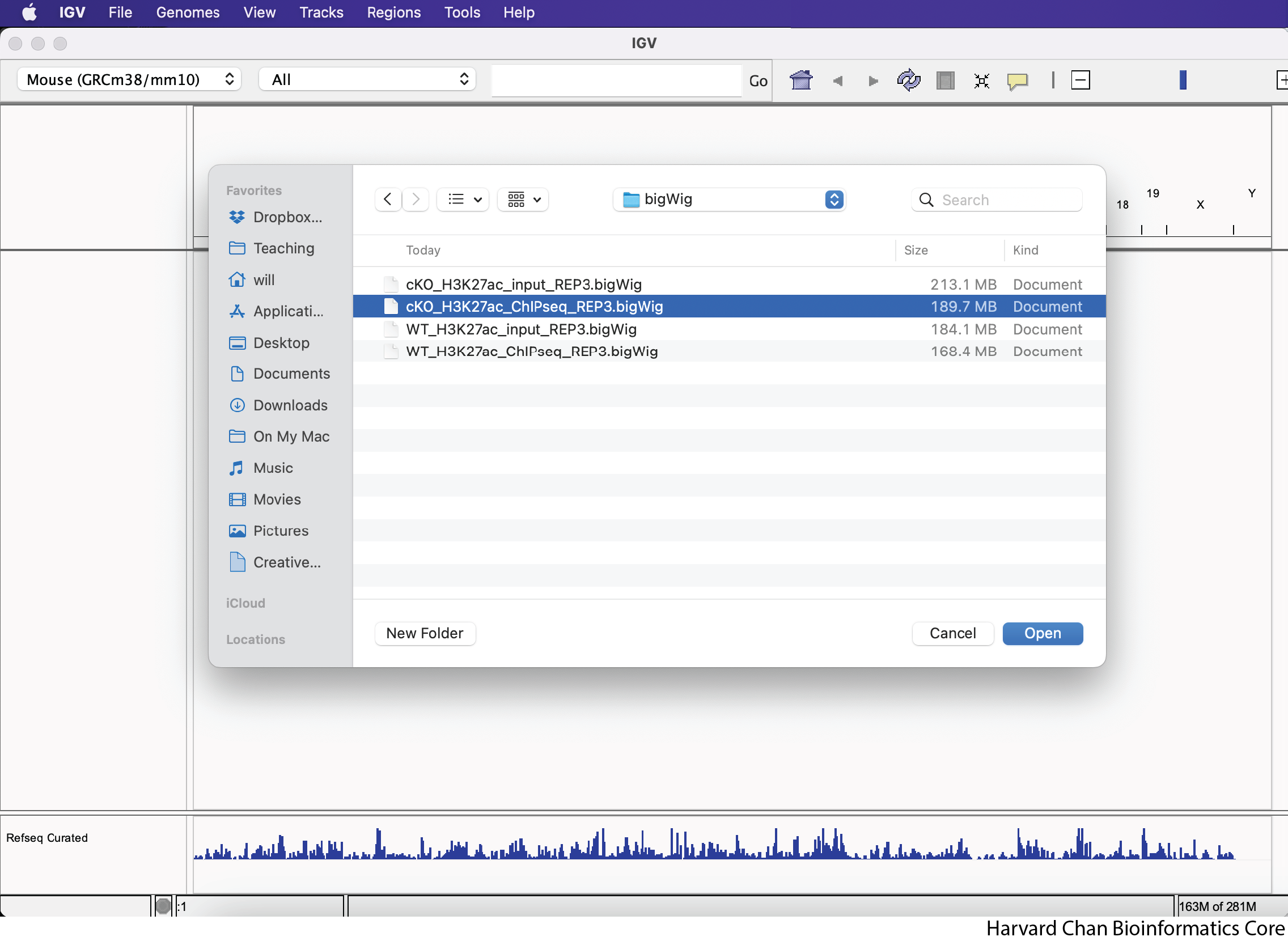
Next, navigate in your file browser to the file you’d like to load, then left-click to select it and left-click “Open”. In this case we are trying to open the file called “cKO_H3K27ac_ChIPseq_REP3.bigWig”, which should be inside your “bigWig” directory within your “data” directory:
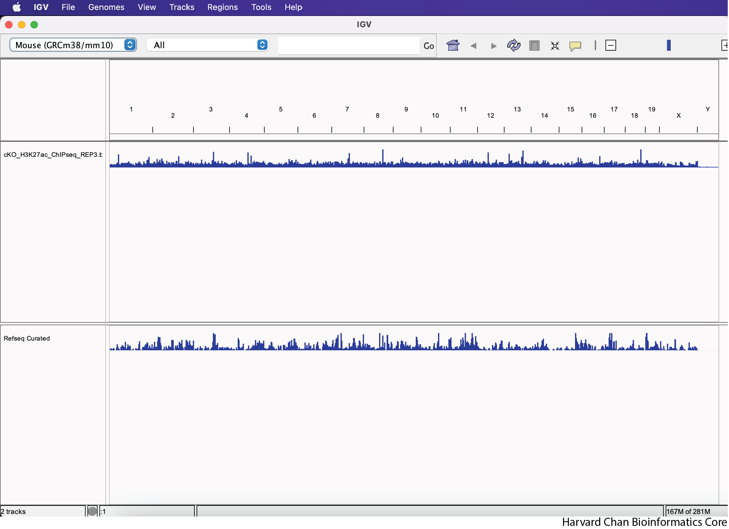
After loading the cKO IP replicate 3 BigWig track, your IGV session should look like:
Loading tracks from URL
Alternatively to loading a track from a local file, we can also load tracks from a URL. In this case, we will load VISTA enhancers that are availible for the Mouse genome on the UCSC Genome Browser. The VISTA enhancers are curated set of computationally predicted and in vivo validated enhancer elements in mouse. The file uses bigBed format, which is used with hosted genome browsers liike the UCSC browser which allows the browser only load the relevant sections of genomes at a time and is less computationally intensive on a public genome browser. More information on bigBed can be found on the UCSC page about bigBed. In order to load a file from a URL, left-click on File in the top-left and select Load from File.... Next, enter this URL into the URL blank:
https://hgdownload.soe.ucsc.edu/gbdb/mm39/vistaEnhancers/vistaEnhancers.bb
Then left-click OK. This process is visualized in the GIF below:
Remove Track
Sometimes you decide that you aren’t interested in a track anymore and you’d like to remove it from you IGV browser. We will remove the “vistaEnhancers.bb” track that we just added. In order to remove a track, right-click on the track and select “Remove Track”. This process is visualized in the GIF below:
Exercise
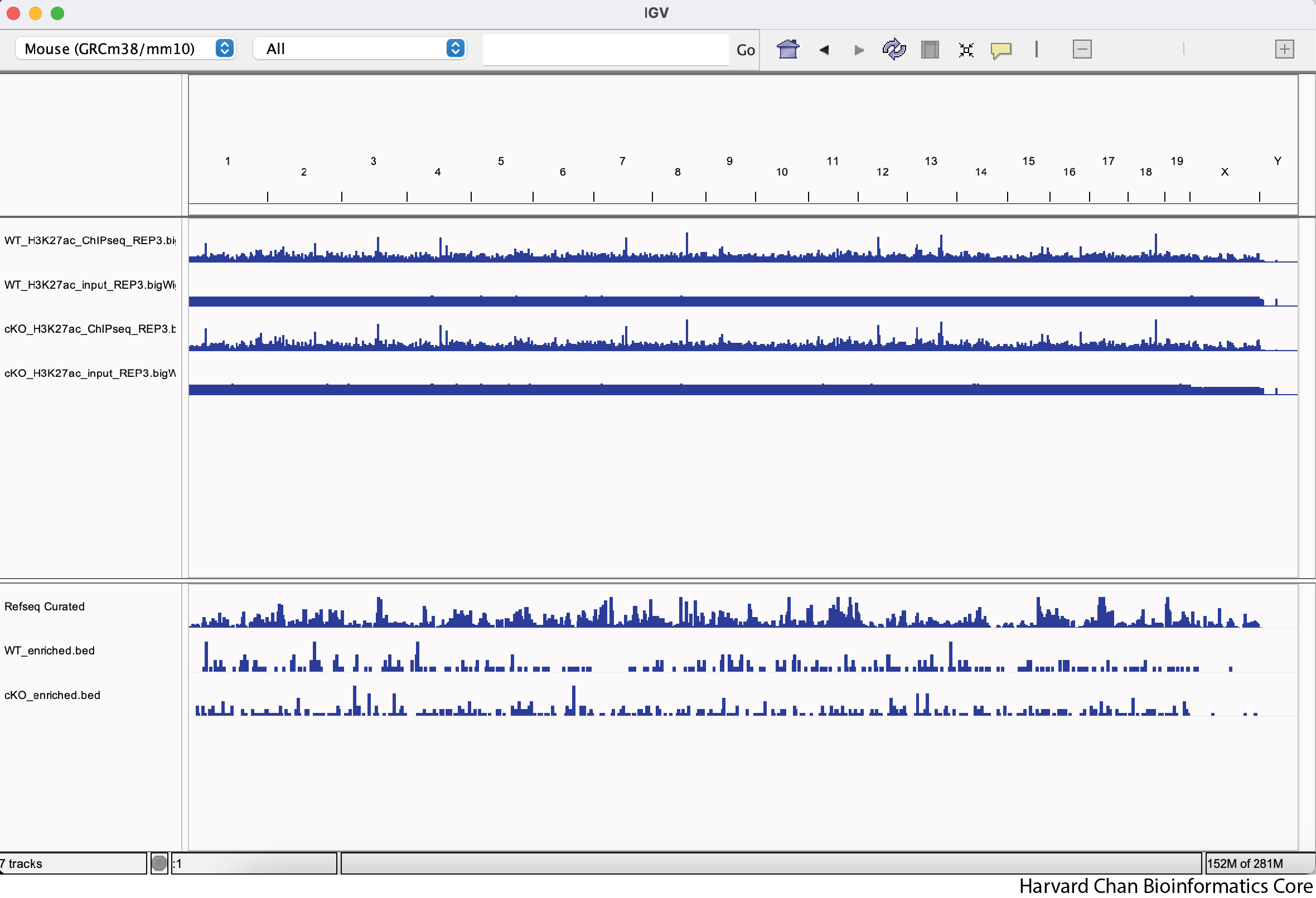
Load the three additional BigWig files you were provided within the “BigWig” directory along with the two BED files within the “DiffBind” directory. Were the BED files loaded in the same area in IGV as the BigWig tracks? If not, where did they load?
Click here to see what your IGV window should look like after loading these files
Note: The order of the track is dependent on the order that you loaded the tracks in, so your track order may be different than in the image below.

Move tracks
Oftentimes, just because you loaded some tracks, that doesn’t mean that they are arranged in the order that you would like them to be in. In order to change the order of the tracks we will left-click on the track where the track’s name is located and drag to move it to where you’d like to see it. This process is visualized in the GIF below:
Exercise
Re-order the tracks so that the WT tracks are above the cKO tracks and the IP samples are above the input samples for their respective experimental condition. Your IGV browser should look like:
There is nothing to submit to the Google Form for this question.
Navigate in IGV
When using IGV it is critical that you are able to navigate to the place in the genome that you are interested in viewing. Below we will discuss a couple of ways to navigate around the genome in the IGV browser.
Zoom in and out on regions
The first way that we can zoom in on a region in IGV is to left-click and hold while dragging over the region we are interested in. This can be iteratively done as one narrows down the region that they are interested in viewing. This process is visualized in the GIF below:
We can zoom in and out using the + and -, respectively, on the right of the top bar. This process is visualized in the GIF below:
Jump to regions
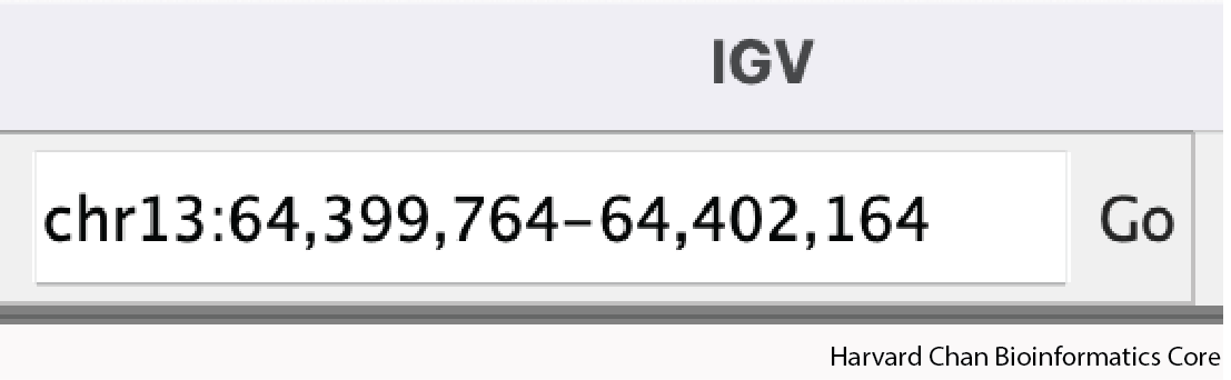
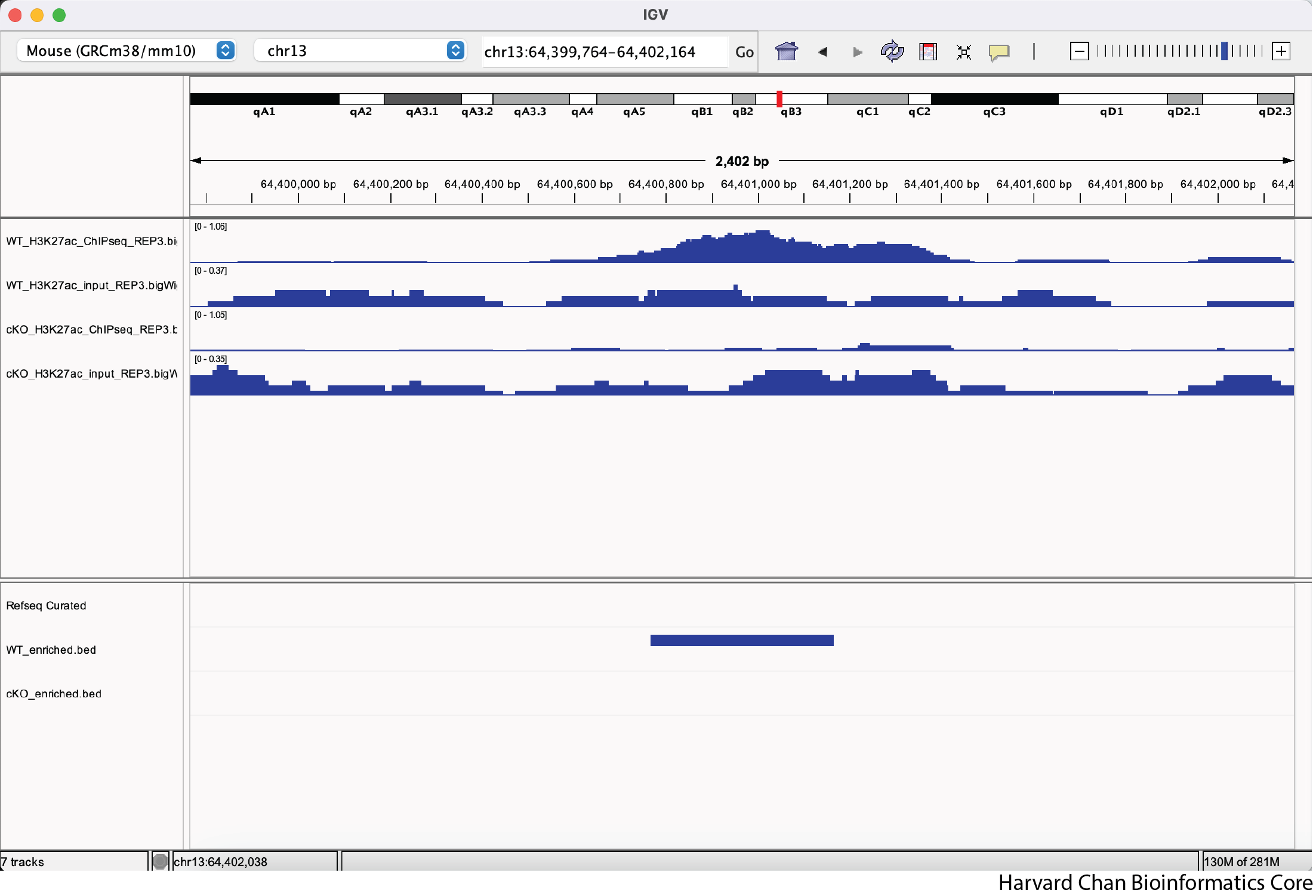
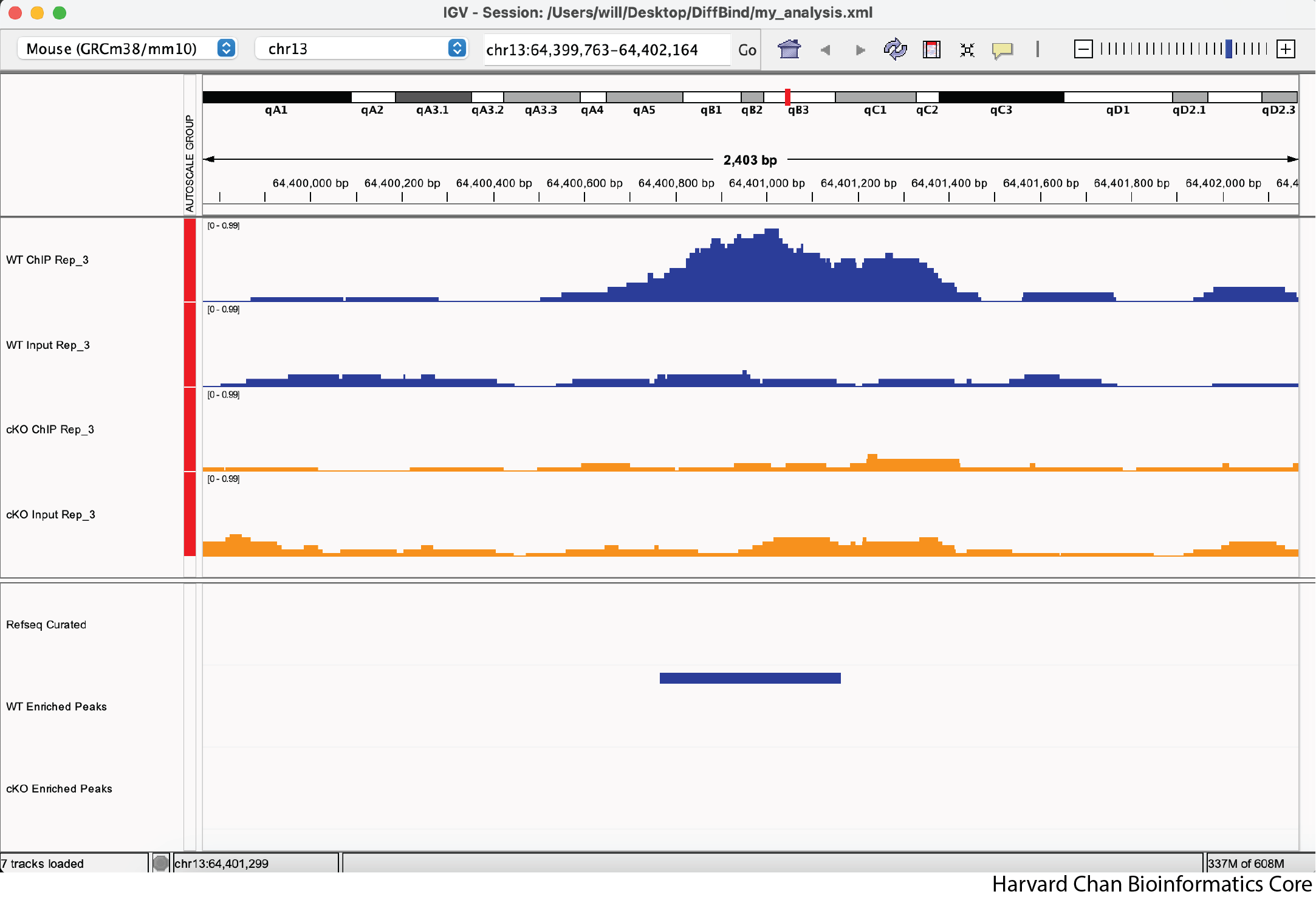
Rather than zooming in on a region, you may already have an idea of where you you would like to analyze and you would like to just jump right to that region. Let’s go to a region where we might want to inspect a peak that DiffBind has informed us has significant differential binding. It is located on Chromosome 13 from 64,400,764 to 64,401,164, but let’s broaden our region by a kilobase on each side in order to give us some context of the genomic landscape around this differentially bound peak. In the genomic coordinates box in the top center of the IGV browser, let’s enter chr13:64,399,764-64,402,164 and left-click “Go”.
The IGV window should look like:
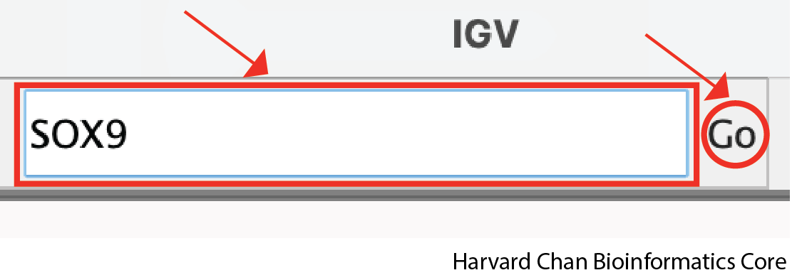
Alternatively, if there is a gene we are particularly interested in going to, we can also enter the gene’s name in this same box and left-click the Go button:
Modify tracks
At this point, we have identified a region that we’d like to investigate, but we need to clean up the aesthetics of this region in order for us to more clearly evaluate this peak, which DiffBind has indicated shows significant differential binding.
Adjust data range
One of the most important steps when comparing between tracks with quantitative ranges like BigWig files is that you’ll need to set the data range to be the same across all tracks. We can look at our IGV browser and look in the top-left of each track (to the right of the track’s name) and we will see the track’s minimum and maximum data range displayed as [Minimum - Maximum].
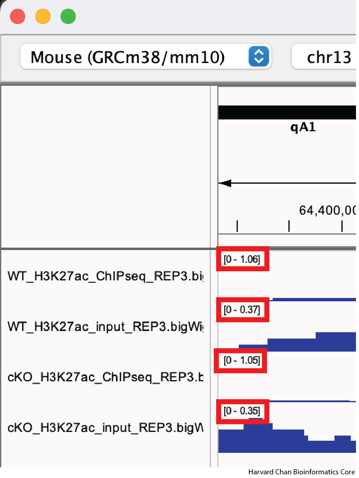
There are two ways to modify a track’s data range:
- Setting each track’s data range manually
- Utilizing IGV’s
Group Autoscalefeature
Setting Data Range Manually
Let’s first look at setting a track’s data range manually. We can to right-click on our top track, WT_H3K27ac_ChIPseq_REP3.bigWig, and select “Set Data Range…” from the dropdown menu:
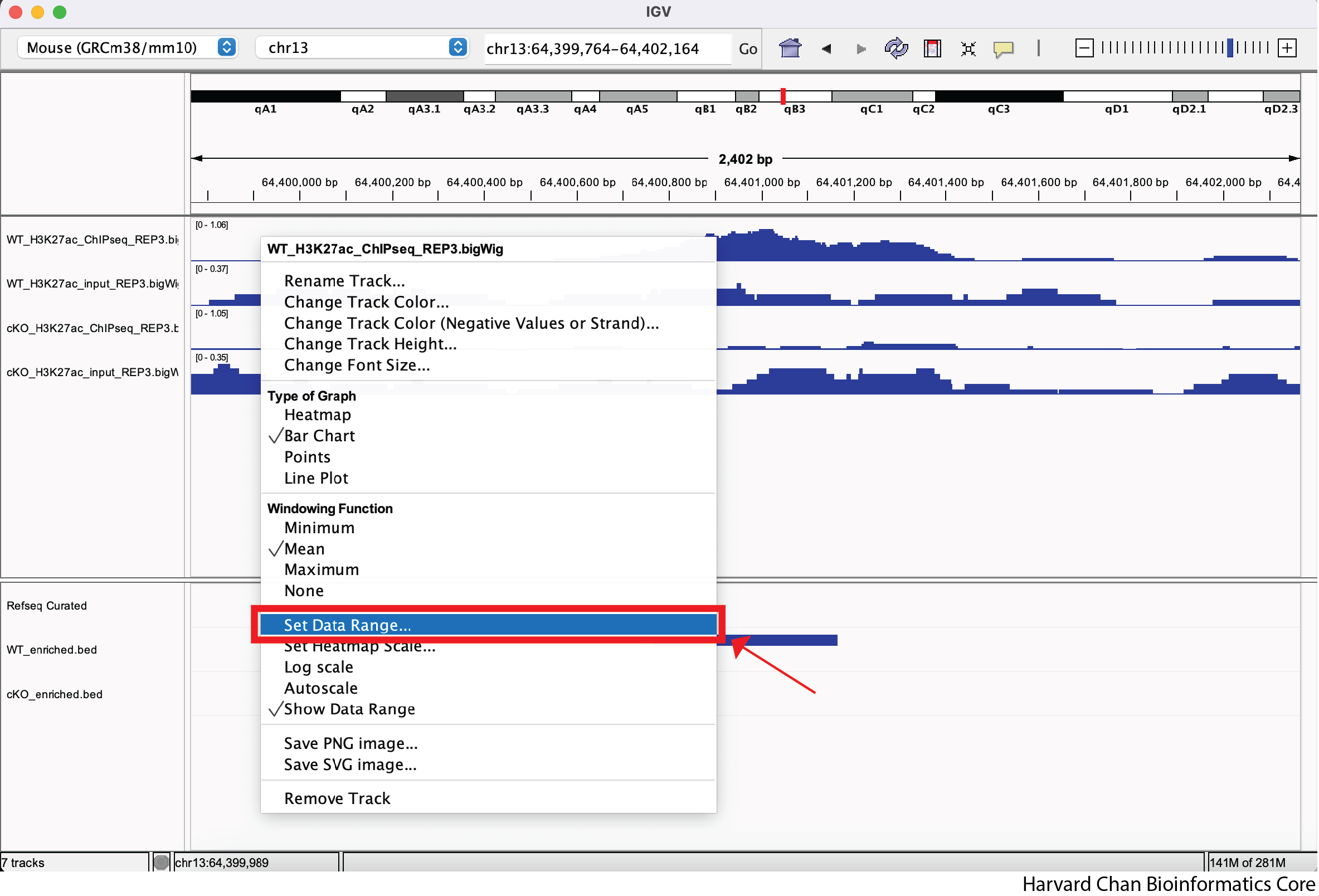
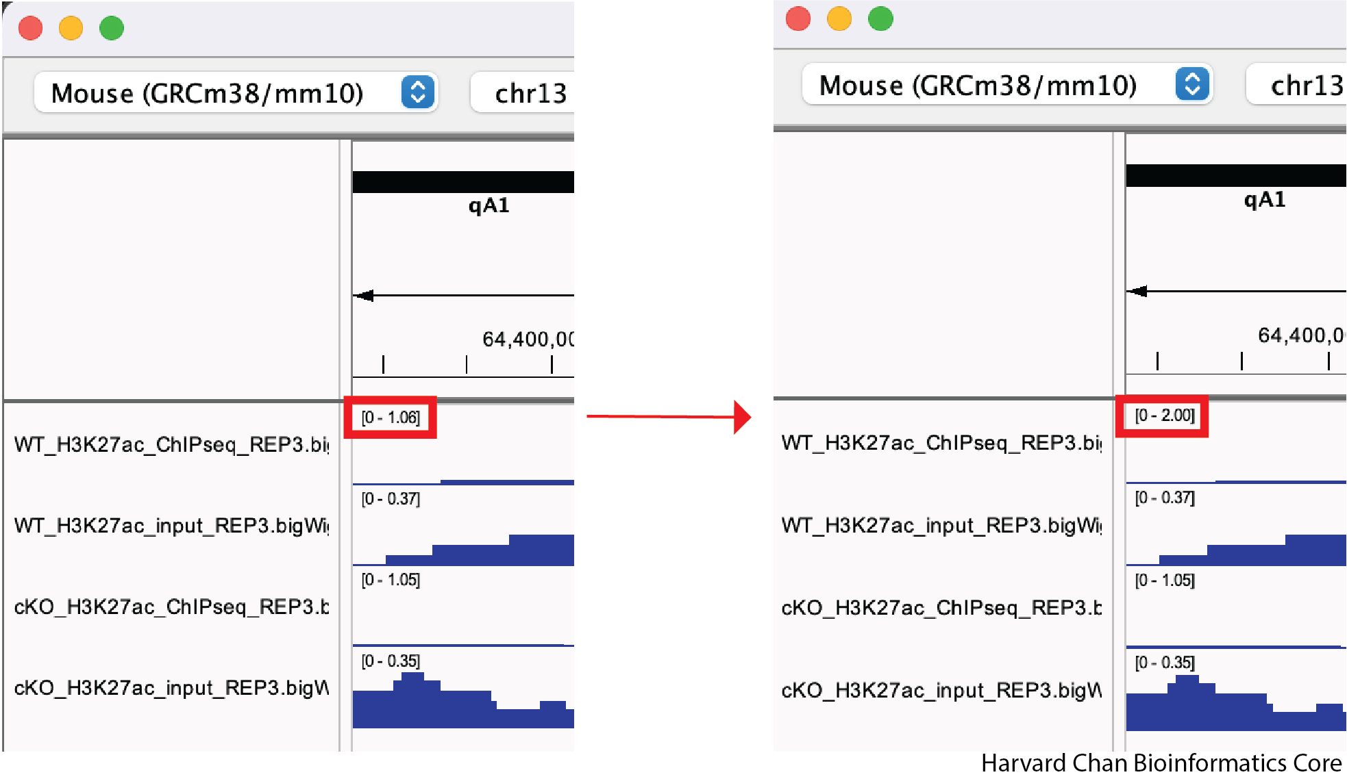
Next, let’s alter the maximum to be 2 and left-click “OK” from the pop-up menu:

If we wanted, we could also alter the minimum value or make our data range be log-scaled from this pop-up menu. We can know see that our track’s data range has changed from [0-1.06] to [0 - 2.00].
Using IGV’s Group Autoscale
While it is nice to be able to adjust a data range, it can be tedious to do it across all of your samples in order to make your sample comparable. Furthermore, if you move to a different location in the genome to look at a different peak, you will likely need to re-adjust your data ranges. Fortunately, IGV has a nifty function called “Group Autoscale” that can help with this. It will:
- Automatically adjust the data range for all of the sample in the group to be the same
- Automatically re-adjust the data range as genomic coordinates change
In order to use the “Group Autoscale” function in IGV you will need to select all of the tracks you would like to group by either:
- Selecting a range of tracks while holding Shift
- Selecting tracks individually while holding Command on MacOS or Ctrl on Windows
Next, right-click in the track names area and select the “Group Autoscale” function. Now, the tracks will be have the same data range and will automatically adjust as the data range changes. This process is visualized in the GIF below:
Adjust track height
We can see in our IGV browser that there is a lot of whitespace that we might like to have our tracks occupy. There are a two ways to adjust the height of the tracks so that they occupy some of the white space. First, we can right-click on a track and select “Change Track Height…”. Then select a new height and left-click “OK”. This process is visualized in the GIF below:
Alternatively, we can use the “Resize tracks to fit in window” button on the top of our IGV browser to resize all of our tracks to take up more of the whitespace. This process is visualized in the GIF below:
Note: If you have too few tracks there still might be some whitespace left and if you have too many it may only squish them to a certain point before offering you the option to scroll down through the tracks.
Adjust color
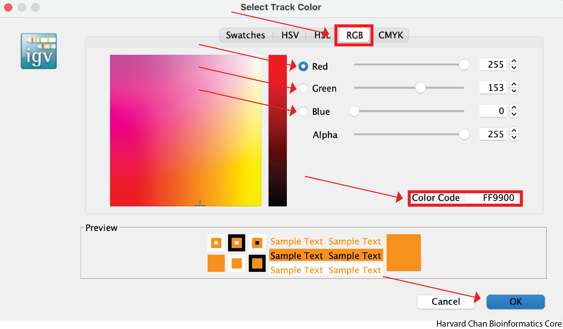
It can be nice to adjust the color in IGV in order to demonstrate contrasts between samples or conditions. Let’s go ahead and change the color of the cKO ChIP sample to orange. Right-click on a track and select “Change Track Color…”. Select the desired color of your track and left-click “OK”. This process is visualized in the GIF below:
However, you may want finer control over your color selection and you can use some of the other tabs to do this. The “RGB” tab allows you to define the level of red, green and blue you want in the color. Of particular note, it also allows you to place the hexadecimal code for the color you want in the “Color Code” text box. For instance, this could be of interest if you are trying to keep consistent colors from other figures where you defined a hexadecimal code for a given dataset. Once you have selected a color that you like, you can left-click the OK button:
Rename Tracks
Oftentimes, the sample names that we use during the processing of our samples are not the most obivious track names to a third party in IGV. Fortunately, we can change the track name in the IGV browser easily. We can right-click on a track and select “Rename Track…”. Enter your new track’s name and left-click the “OK” button. Let’s rename the “cKO_H3K27ac_ChIPseq_REP3.bigWig” to be “cKO ChIP Rep_3”. This process is visualized in the GIF below:
Saving and Loading IGV Sessions
Oftentimes, you’ll want to save your IGV session or load up an IGV session that you’ve been previously working on. Below we will describe how to save and load IGV sessions.
Saving an IGV Session
Now that you have edited your tracks to get them just the way you want you them, you might want to save the IGV session so that you can easily reload it for when you want to revisit it. To save your IGV session, go to the top bar and left-click File → Save Session.... Then name your session and left-click “OK”. You can notice that the name and path to the session is now at the top of the IGV browser.
After saving our IGV session, let’s close IGV.
Loading an IGV Session
If we now open IGV back up, we will notice that it provides a fresh session. If we want to pick-up our analysis where we left off our previous IGV session, we will need to load the previous session. To load an IGV session, go to the top bar and left-click File → Open Session.... Navigate to the desired IGV session and left-click “Open”. Now the previous IGV session should be loaded where you left off.
It is VERY IMPORTANT that if you move files that were loaded into IGV into a different location on your computer, IGV will not be able to find them and therefore not load your saved session!
Exercise
1) Now that we’ve explored some of the functionality from IGV let’s format our IGV browser and qualitatively assess some regions in the genome.
a. Rename “cKO_H3K27ac_input_REP3.bigWig” to “cKO Input Rep_3”
b. Rename “WT_H3K27ac_ChIPseq_REP3.bigWig” to “WT ChIP Rep_3”
c. Rename “WT_H3K27ac_input_REP3.bigWig” to “WT Input Rep_3”
d. Rename “WT_enriched.bed” to “WT Enriched Peaks”
e. Rename “cKO_enriched.bed” to “cKO Enriched Peaks”
Click here to see what the IGV session should look like
There is nothing to submit to the Google Form for this question.
2) Change the color of the “cKO Input Rep_3” and “cKO Enriched Peaks” tracks to orange
Click here to see what the IGV session should look like
There is nothing to submit to the Google Form for this question.
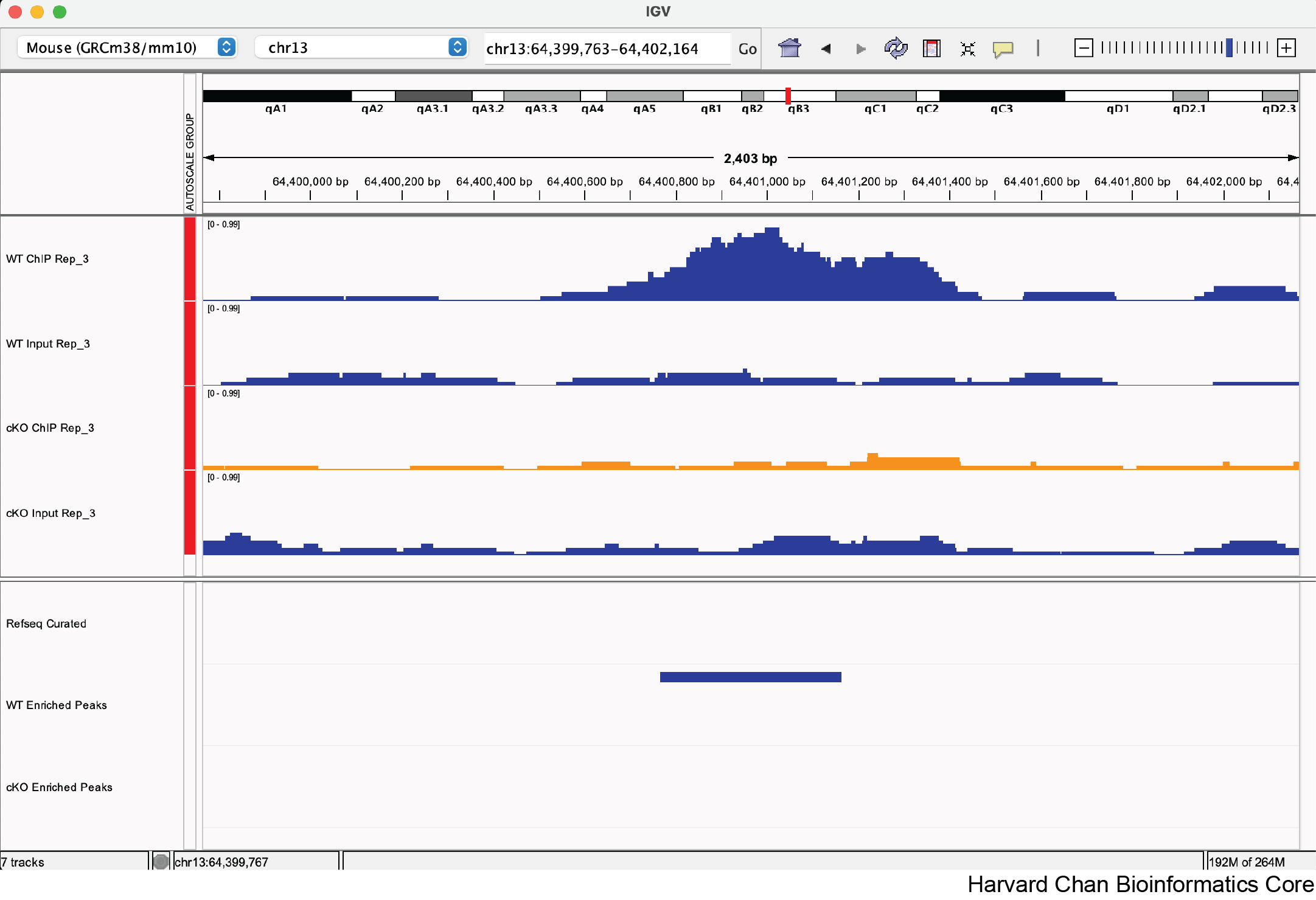
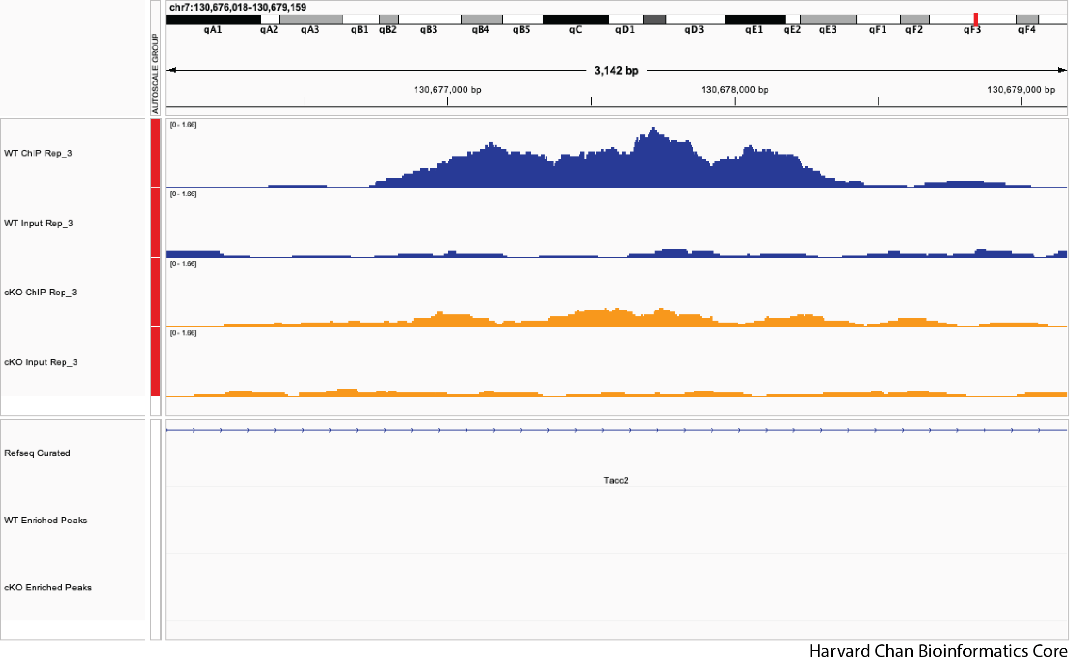
3) Let’s explore a few regions and see if we qualitatively agree with DiffBind’s analysis. Do you agree with DiffBind’s call or non-call differentially bound peak for the following genomic coordinates:
a. chr13:64,400,764-64,401,164
b. chr1:131,492,210-131,492,610
c. chr7:130,677,389-130,677,789
Note: The FDR for this peak is 0.051
Save Image
Lastly, now that we’ve completed an analysis we might be interested in saving an image of our analysis. You can either take a screenshot or use the built-in capabilities of IGV to save an image. In order to save an image, left-click File → Save PNG Image.../Save SVG Image.... Name the image and left-click “Save”. This process is visualized in the GIF below:
This image will look like:
This lesson has been developed by members of the teaching team at the Harvard Chan Bioinformatics Core (HBC). These are open access materials distributed under the terms of the Creative Commons Attribution license (CC BY 4.0), which permits unrestricted use, distribution, and reproduction in any medium, provided the original author and source are credited.