Contributors: Meeta Mistry, Radhika Khetani, Jihe Liu, Mary Piper, Will Gammerdinger

Approximate time: 30 minutes

Learning Objectives

• Differentiate between the different file formats available for peak visualization
• Create bigWig files using deepTools

Peak visualization

Now that we have identified regions in the genome that are enriched through some interaction with PRDM16, we can take those regions and visually assess the amount of signal observed. This can be done in one of two ways:

1. Uploading the data to a genome viewer such as the Broad’s Integrative Genome Viewer (IGV) or the UCSC Genome Browser, to explore the genome and specific loci for pileups.
2. Create profile plots and heatmaps to look at the signal aggregated over all binding sites.

In order to perform any of assessments described above, you will need a file in the appropriate format.

The goal of this lesson is to introduce you to different file formats used for ChIP-seq data visualization and how to generate these files using deepTools.

File formats for peak visualization

There are several different types of file formats that can hold data associated with high-throughput sequencing data, these file formats have a distinct structure and hold specific types of data. We have already encountered:

• the sequence data format - FASTQ
• the alignment file formats - SAM and BAM
• the peak call format - BED, narrowPeak

In this section we want to introduce you to a few additional formats that can be used for visualizing peaks.

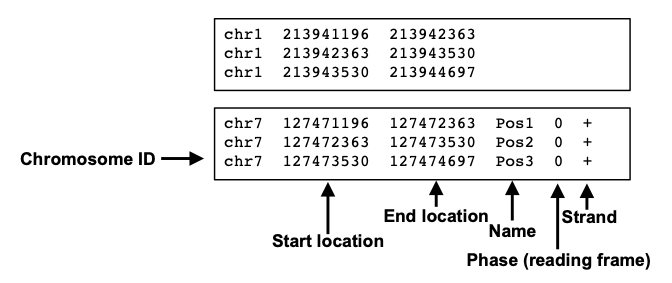
The commonality among these file formats is that they represent the peak location in a manner similar to the BED format (shown below).

BedGraph format

In addition to accomodating peak calls (discrete data), the BedGraph format also allows display of continuous data as a track on a genome browser. This display type is useful for including and plotting some quantitative information, e.g. intensity. For the purposes of visualization, bedGraph and bigWig are pratically interchangeable, with the bigWig file being a lot smaller for a given dataset.

Wiggle and bigWig formats

The Wiggle format (wig) also allows the display of continuous data. This format is “line” oriented, and has declaration lines and data lines. It also requires a separate wiggle track definition line as a header. There are two options for how data in wiggle files are represented: variableStep and fixedStep. These formats were developed to allow the file to be written as compactly as possible.

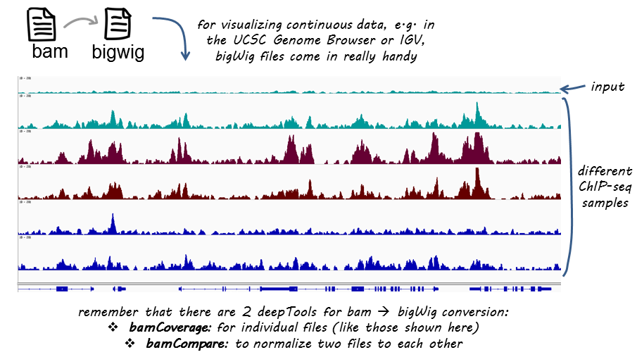
The bigWig format is an indexed binary form of the wiggle file format, and is useful for large amounts of dense and continuous data to be displayed in a genome browser as a graphical track. As mentioned above, the visual representation of this format is very similar to bedGraph.

NOTE: All of the above file formats are also applicable to CUT&RUN and ATAC-seq data.

Creating bigWig files

For this workshop, we will focus on creating bigWig files, as we will be using them in the next lesson for qualitative assessment. BigWig files have a much smaller data footprint compared to BAM files, especially as your bin size (a parameter described below) increases. The general procedure is to take our alignment files (BAM) and convert them into bigWig files, and we will do this using deepTools. The coverage is calculated as the number of reads per bin, where bins are short consecutive counting windows of a defined size. It is possible to extended the length of the reads to better reflect the actual fragment length.

Image acquired from the deepTools documentation

deepTools is a suite of Python tools developed for the efficient analysis of high-throughput sequencing data, such as ChIP-seq, RNA-seq, or MNase-seq. deepTools has a wide variety of commands that go beyond what we will cover in this workshop. We encourage you to look through the documentation and explore more on your own time.

Setting up

The command for creating a bigWig file is fairly computationally heavy and so we will make use of the muti-threading functionality in deepTools. This means that we will also need to request more cores for our interactive session. If you are already logged on to a compute node, you will need to exit and start a new session. Note that we will ask for 6 cores, and also increase our memory to 8G.

$ srun --pty -p interactive -t 0-12:00 --mem 8G -c 6 /bin/bash

Once on a compute node, begin by creating a directory for the output.

$ cd ~/chipseq_workshop/results/
$ mkdir -p visualization/bigWig

We then need to create an index file for the BAM file. Often, when working with BAM files you will find that many tools require an index (an associated .bai file). You can think of an index similar to that which is located at the back of a textbook - when you are interested in a particular subject, you look for the keyword in the index and identify the pages that contain the relevant information. Similarily, indexing the BAM file aims to achieve fast retrieval of alignments overlapping a specified region without going through the whole alignment file. Essentially, a bai file along with the bam ensures that downstream applications are able to use the information with the bam file much more speedily.

We will use SAMtools again, specifically the samtools index command, to index the BAM file.

Let’s load the samtools module:

$ module load gcc/6.2.0 samtools/1.13

Create an index for the wt_sample2_chip_final.bam file that we created in earlier lesson:

$ samtools index ~/chipseq_workshop/results/bowtie2/wt_sample2_chip_final.bam

Check your bowtie2 folder to make sure see the new index file that was generated!

Finally, let’s make sure we have the required modules loaded to use deepTools:

$ module load python/2.7.12 deeptools/3.0.2 

Normalization

The methods for bigWig creation (bamCoverage and bamCompare) allows for normalization, which is great if we want to compare different samples to each other and they vary in terms of sequencing depth. DeepTools offers different methods of normalization as listed below, each is perfomed per bin. The default is no normalization.

NOTE: We will not normalize the data we are working with because we are following the methods described in Baizabal, 2018. However, it is highly recommended to choose one of the methods described.

• Reads Per Kilobase per Million mapped reads (RPKM)
  • number of reads per bin / (number of mapped reads (in millions) * bin length (kb))
• Counts per million (CPM); this is similar to CPM in RNA-seq
  • number of reads per bin / number of mapped reads (in millions)
• Bins Per Million mapped reads (BPM); same as TPM in RNA-seq
  • number of reads per bin / sum of all reads per bin (in millions)
• Reads per genomic content (RPGC)
  • number of reads per bin / scaling factor for 1x average coverage
  • scaling factor is determined from the sequencing depth: total number of mapped reads * fragment length) / effective genome size
  • this option requires an effectiveGenomeSize

Spike-in normalization

Another option for normalization is to normalize each sample using a scale factor/ normalization factor. By default the scale factor is set to 1 in deepTools. In an earlier lesson, we described the spike-in strategy and how to compute a normalization factor for each indidvidual sample. Those values can be used when creating bigWig files. The --scaleFactor parameter takes in the user provided value and each bin is multiplied by this value. If normalizing with a scale factor, be sure that none of the other normalization methods are applied.

NOTE: The scaleFactor is not applicable to ATAC-seq data, as the spike-in strategy is not used.

bamCoverage from deepTools

This command takes a BAM file as input and evaluates which areas of the genome have reads associated with them, i.e. how much of the genome is “covered” with reads. The coverage is calculated as the number of reads per bin, where bins are short consecutive sections of the genome (bins) that can be defined by the user. The output of this command can be either a bedGraph or a bigWig file. We will be generating a bigWig file, since that format has a much smaller data footprint, especially as the bin size increases.

These are some parameters of bamCoverage that are worth considering:

• normalizeUsing: Possible choices: RPKM, CPM, BPM, RPGC. By default, no normalization is applied.
• binSize: size of bins in bases (default is 50)
• --effectiveGenomeSize: the portion of the genome that is mappable. It is useful to consider this when computing your scaling factor.
• smoothLength: defines a window, larger than the binSize, to average the number of reads over. This helps produce a more continuous plot.
• centerReads: reads are centered with respect to the fragment length as specified by extendReads. This option is useful to get a sharper signal around enriched regions.

We will be using the bare minimum of parameters as shown in the code below. We decrease the bin size to increase the resolution of the track (this also means larger file size). If you are interested, feel free to test out some of the other parameters to create different bigWig files. You can load them into a genome viewer like IGV and observe the differences.

Let’s create a bigWig file for wt_sample2_chip, with a binSize of 20.

$ bamCoverage -b ~/chipseq_workshop/results/bowtie2/wt_sample2_chip_final.bam \
-o ~/chipseq_workshop/results/visualization/bigWig/wt_sample2_chip.bw \
--binSize 20

Note: This command can take up to 10 minutes to complete.

bamCompare from deepTools

As an alternate to calculating genome coverage with bamCoverage, we could use bamCompare. bamCompare will create a bigWig file in which we compare the ChIP against the input. The command is quite similar to bamCoverage, except that it requires two files as input (b1 and b2). Below, we show you an example of how you would run bamCompare. The default --operation used to compare the two samples is the log2 ratio, however you also have the option to add, subtract and average. Any of the parameters described above for bamCoverage can also be used.

## DO NOT RUN

$ bamCompare -b1 ~/chipseq_workshop/results/bowtie2/wt_sample2_chip_final.bam \
-b2 ~/chipseq_workshop/results/bowtie2/wt_sample2_input_final.bam \
-o ~/chipseq_workshop/results/visualization/bigWig/wt_sample2_chip.bw \
--binSize 20

You can find more details about the difference between bamCompare and bamCoverage linked here.

---

This lesson has been developed by members of the teaching team at the Harvard Chan Bioinformatics Core (HBC). These are open access materials distributed under the terms of the Creative Commons Attribution license (CC BY 4.0), which permits unrestricted use, distribution, and reproduction in any medium, provided the original author and source are credited.