Approximate time: 50 min
Learning Objectives
- Describe and utilize functions in R.
- Modify default behavior of functions using arguments in R.
- Identify R-specific sources of help to get more information about functions.
- Demonstrate how to create user-defined functions in R
- Demonstrate how to install external packages to extend R’s functionality.
- Identify different R-specific and external sources of help to (1) troubleshoot errors and (2) get more information about functions and packages.
Functions and their arguments
What are functions?
A key feature of R is functions. Functions are “self contained” modules of code that accomplish a specific task. Functions usually take in some sort of data structure (value, vector, dataframe etc.), process it, and return a result.
The general usage for a function is the name of the function followed by parentheses:
function_name(input)
The input(s) are called arguments, which can include:
- the physical object (any data structure) on which the function carries out a task
- specifications that alter the way the function operates (e.g. options)
Not all functions take arguments, for example:
getwd()
However, most functions can take several arguments. If you don’t specify a required argument when calling the function, you will either receive an error or the function will fall back on using a default.
The defaults represent standard values that the author of the function specified as being “good enough in standard cases”. An example would be what symbol to use in a plot. However, if you want something specific, simply change the argument yourself with a value of your choice.
Basic functions
We have already used a few examples of basic functions in the previous lessons i.e getwd(), c(), and factor(). These functions are available as part of R’s built in capabilities, and we will explore a few more of these base functions below.
You can also get functions from external packages or libraries, or even write your own. We will take a closer look at both of these soon!
Let’s revisit a function that we have used previously to combine data c() into vectors. The arguments it takes is a collection of numbers, characters or strings (separated by a comma). The c() function performs the task of combining the numbers or characters into a single vector. You can also use the function to add elements to an existing vector:
glengths <- c(glengths, 90) # adding at the end
glengths <- c(30, glengths) # adding at the beginning
What happens here is that we take the original vector glengths (containing three elements), and we are adding another item to either end. We can do this over and over again to build a vector or a dataset.
Since R is used for statistical computing, many of the base functions involve mathematical operations. One example would be the function sqrt(). The input/argument must be a number, and the output is the square root of that number. Let’s try finding the square root of 81:
sqrt(81)
Now what would happen if we called the function (e.g. ran the function), on a vector of values instead of a single value?
sqrt(glengths)
In this case the task was performed on each individual value of the vector glengths and the respective results were displayed.
Let’s try another function, this time using one that we can change some of the options (arguments that change the behavior of the function), for example round:
round(3.14159)
We can see that we get 3. That’s because the default is to round to the nearest whole number. What if we want a different number of significant digits?
Seeking help on arguments for functions
The best way of finding out this information is to use the ? followed by the name of the function. Doing this will open up the help manual in the bottom right panel of RStudio that will provide a description of the function, usage, arguments, details, and examples:
?round
Alternatively, if you are familiar with the function but just need to remind yourself of the names of the arguments, you can use:
args(round)
Even more useful is the example() function. This will allow you to run the examples section from the Online Help to see exactly how it works when executing the commands. Let’s try that for round():
example("round")
In our example, we can change the number of digits returned by adding an argument. We can type digits=2 or however many we may want:
round(3.14159, digits=2)
NOTE: If you provide the arguments in the exact same order as they are defined (in the help manual) you don’t have to name them:
round(3.14159, 2)However, it’s usually not recommended practice because it involves a lot of memorization. In addition, it makes your code difficult to read for your future self and others, especially if your code includes functions that are not commonly used. (It’s however OK to not include the names of the arguments for basic functions like
mean,min, etc…). Another advantage of naming arguments, is that the order doesn’t matter. This is useful when a function has many arguments.
Exercise
- Another commonly used base function is
mean(). Use this function to calculate an average for theglengthsvector. - Use the help manual to identify additional arguments for
mean().
Missing values
By default, all R functions operating on vectors that contains missing data will return NA. It’s a way to make sure that users know they have missing data, and make a conscious decision on how to deal with it. When dealing with simple statistics like the mean, the easiest way to ignore
NA(the missing data) is to usena.rm=TRUE(rmstands for remove).In some cases, it might be useful to remove the missing data from the vector. For this purpose, R comes with the function
na.omitto generate a vector that has NA’s removed. For some applications, it’s useful to keep all observations, for others, it might be best to remove all observations that contain missing data. The functioncomplete.cases()returns a logical vector indicating which rows have no missing values.
User-defined Functions
One of the great strengths of R is the user’s ability to add functions. Sometimes there is a small task (or series of tasks) you need done and you find yourself having to repeat it multiple times. In these types of situations it can be helpful to create your own custom function. The structure of a function is given below:
name_of_function <- function(argument1, argument2) {
    statements or code that does something
    return(something)
}
- First you give your function a name.
- Then you assign value to it, where the value is the function.
When defining the function you will want to provide the list of arguments required (inputs and/or options to modify behaviour of the function), and wrapped between curly brackets place the tasks that are being executed on/using those arguments. The argument(s) can be any type of object (like a scalar, a matrix, a dataframe, a vector, a logical, etc), and it’s not necessary to define what it is in any way.
Finally, you can “return” the value of the object from the function, meaning pass the value of it into the global environment. The important idea behind functions is that objects that are created within the function are local to the environment of the function – they don’t exist outside of the function.
NOTE: You can also have a function that doesn’t require any arguments, nor will it return anything.
Let’s try creating a simple example function. This function will take in a numeric value as input, and return the squared value.
square_it <- function(x) {
    square <- x * x
    return(square)
}
Now, we can use the function as we would any other function. We type out the name of the function, and inside the parentheses we provide a numeric value x:
square_it(5)
Pretty simple, right? In this case, we only had one line of code that was run, but in theory you could have many lines of code to get obtain the final results that you want to “return” to the user. We have only scratched the surface here when it comes to creating functions! We will revisit this in later lessons, but if interested you can also find more detailed information on this R-bloggers site, which is where we adapted this example from.
Packages and Libraries
Packages are collections of R functions, data, and compiled code in a well-defined format, created to add specific functionality. There are 10,000+ user contributed packages and growing.
There are a set of standard (or base) packages which are considered part of the R source code and automatically available as part of your R installation. Base packages contain the basic functions that allow R to work, and enable standard statistical and graphical functions on datasets; for example, all of the functions that we have been using so far in our examples.
The directories in R where the packages are stored are called the libraries. The terms package and library are sometimes used synonymously and there has been discussion amongst the community to resolve this. It is somewhat counter-intuitive to load a package using the library() function and so you can see how confusion can arise.
You can check what libraries are loaded in your current R session by typing into the console:
sessionInfo() #Print version information about R, the OS and attached or loaded packages

# OR

search() #Gives a list of attached packages
In this workshop we have introduced you to functions from the standard base packages. However, the more you work with R you will come to realize that there is a cornucopia of R packages that offer a wide variety of functionality. To use additional packages will require installation. Many packages can be installed from the CRAN or Bioconductor repositories.
Package installation from CRAN
CRAN is a repository where the latest downloads of R (and legacy versions) are found in addition to source code for thousands of different user contributed R packages.
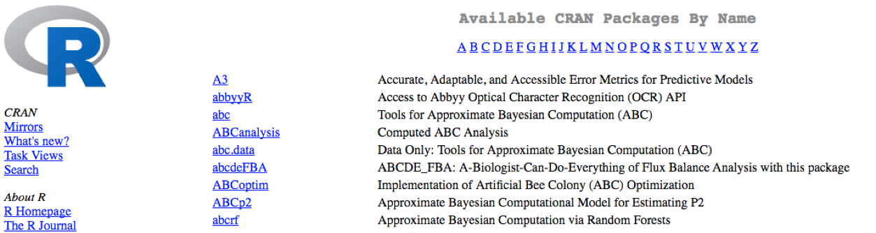
Packages for R can be installed from the CRAN package repository using the install.packages function. This function will download the source code from on the CRAN mirrors and install the package (and any dependencies) locally on your computer.
An example is given below for the ggplot2 package that will be required for some plots we will create later on. Run this code to install ggplot2.
install.packages("ggplot2")
Package installation from Bioconductor
Alternatively, packages can also be installed from Bioconductor, another repository of packages which provides tools for the analysis and comprehension of high-throughput genomic data. These packages includes (but is not limited to) tools for performing statistical analysis, annotation packages, and accessing public datasets.
![]()
There are many packages that are available in CRAN and Bioconductor, but there are also packages that are specific to one repository. Generally, you can find out this information with a Google search or by trial and error.
To install from Bioconductor, you will first need to install BiocManager. This only needs to be done once ever for your R installation.
# DO NOT RUN THIS!

install.packages("BiocManager")
Now you can use the install() function from the BiocManager package to install a package by providing the name in quotations.
Here we have the code to install ggplot2, through Bioconductor:
# DO NOT RUN THIS!

BiocManager::install("ggplot2")
The code above may not be familiar to you - it is essentially using a new operator, a double colon
::to execute a function from a particular package. This is the syntax:package::function_name().
Package installation from source
Finally, R packages can also be installed from source. This is useful when you do not have an internet connection (and have the source files locally), since the other two methods are retrieving the source files from remote sites.
To install from source, we use the same install.packages function but we have additional arguments that provide specifications to change from defaults:
# DO NOT RUN THIS!

install.packages("~/Downloads/ggplot2_1.0.1.tar.gz", type="source", repos=NULL)
Loading libraries
Once you have the package installed, you can load the library into your R session for use. Any of the functions that are specific to that package will be available for you to use by simply calling the function as you would for any of the base functions. Note that quotations are not required here.
library(ggplot2)
You can also check what is loaded in your current environment by using sessionInfo() or search() and you should see your package listed as:
other attached packages:
[1] ggplot2_2.0.0
In this case there are several other packages that were also loaded along with ggplot2.
We only need to install a package once on our computer. However, to use the package, we need to load the library every time we start a new R/RStudio environment. You can think of this as installing a bulb versus turning on the light.

Analogy and image credit to Dianne Cook of Monash University.
Finding functions specific to a package
This is your first time using ggplot2, how do you know where to start and what functions are available to you? One way to do this, is by using the Package tab in RStudio. If you click on the tab, you will see listed all packages that you have installed. For those libraries that you have loaded, you will see a blue checkmark in the box next to it. Scroll down to ggplot2 in your list:
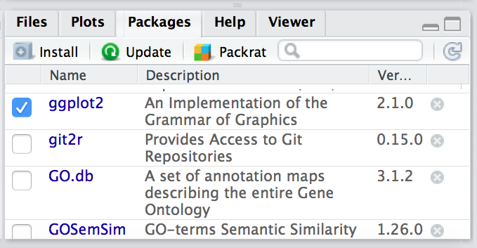
If your library is successfully loaded you will see the box checked, as in the screenshot above. Now, if you click on ggplot2 RStudio will open up the help pages and you can scroll through.
An alternative is to find the help manual online, which can be less technical and sometimes easier to follow. For example, this website is much more comprehensive for ggplot2 and is the result of a Google search. Many of the Bioconductor packages also have very helpful vignettes that include comprehensive tutorials with mock data that you can work with.
If you can’t find what you are looking for, you can use the rdocumention.org website that search through the help files across all packages available.
Exercise
The ggplot2 package is part of the tidyverse suite of integrated packages which was designed to work together to make common data science operations more user-friendly. We will be using the tidyverse suite in later lessons, and so let’s install it. NOTE: This suite of packages is only available in CRAN.
Asking for help
The key to getting help from someone is for them to grasp your problem rapidly. You should make it as easy as possible to pinpoint where the issue might be.
-
Try to use the correct words to describe your problem. For instance, a package is not the same thing as a library. Most people will understand what you meant, but others have really strong feelings about the difference in meaning. The key point is that it can make things confusing for people trying to help you. Be as precise as possible when describing your problem.
-
Always include the output of
sessionInfo()as it provides critical information about your platform, the versions of R and the packages that you are using, and other information that can be very helpful to understand your problem.sessionInfo() #This time it is not interchangeable with search() -
If possible, reproduce the problem using a very small
data.frameinstead of your 50,000 rows and 10,000 columns one, provide the small one with the description of your problem. When appropriate, try to generalize what you are doing so even people who are not in your field can understand the question.-
To share an object with someone else, you can provide either the raw file (i.e., your CSV file) with your script up to the point of the error (and after removing everything that is not relevant to your issue). Alternatively, in particular if your questions is not related to a
data.frame, you can save any other R data structure that you have in your environment to a file:# DO NOT RUN THIS! save(iris, file="/tmp/iris.RData")The content of this
.RDatafile is not human readable and cannot be posted directly on stackoverflow. It can, however, be emailed to someone who can read it with this command:# DO NOT RUN THIS! some_data <- load(file="~/Downloads/iris.RData")
-
Where to ask for help?
- Google is often your best friend for finding answers to specific questions regarding R.
- Cryptic error messages are very common in R - it is very likely that someone else has encountered this problem already! Start by googling the error message. However, this doesn’t always work because often, package developers rely on the error catching provided by R. You end up with general error messages that might not be very helpful to diagnose a problem (e.g. “subscript out of bounds”).
- Stackoverflow: Search using the
[r]tag. Most questions have already been answered, but the challenge is to use the right words in the search to find the answers: http://stackoverflow.com/questions/tagged/r. If your question hasn’t been answered before and is well crafted, chances are you will get an answer in less than 5 min. - Your friendly colleagues: if you know someone with more experience than you, they might be able and willing to help you.
- The R-help: it is read by a lot of people (including most of the R core team), a lot of people post to it, but the tone can be pretty dry, and it is not always very welcoming to new users. If your question is valid, you are likely to get an answer very fast but don’t expect that it will come with smiley faces. Also, here more than everywhere else, be sure to use correct vocabulary (otherwise you might get an answer pointing to the misuse of your words rather than answering your question). You will also have more success if your question is about a base function rather than a specific package.
- The Bioconductor support site. This is very useful and if you tag your post, there is a high likelihood of getting an answer from the developer.
- If your question is about a specific package, see if there is a mailing list
for it. Usually it’s included in the DESCRIPTION file of the package that can
be accessed using
packageDescription("name-of-package"). You may also want to try to email the author of the package directly. - There are also some topic-specific mailing lists (GIS, phylogenetics, etc…), the complete list is here.
More resources
- The Posting Guide for the R mailing lists.
- How to ask for R help useful guidelines
- The Introduction to R can also be dense for people with little programming experience but it is a good place to understand the underpinnings of the R language.
- The R FAQ is dense and technical but it is full of useful information.
This lesson has been developed by members of the teaching team at the Harvard Chan Bioinformatics Core (HBC). These are open access materials distributed under the terms of the Creative Commons Attribution license (CC BY 4.0), which permits unrestricted use, distribution, and reproduction in any medium, provided the original author and source are credited.
- The materials used in this lesson are adapted from work that is Copyright © Data Carpentry (http://datacarpentry.org/). All Data Carpentry instructional material is made available under the Creative Commons Attribution license (CC BY 4.0).