Approximate time: 60 minutes
Learning Objectives
- Annotating peaks with gene and genomic feature information
- Obtaining biological context for identified binding sites using functional enrichment tools
- Using the seqqunce data for peaks to identify possible over-represented motifs
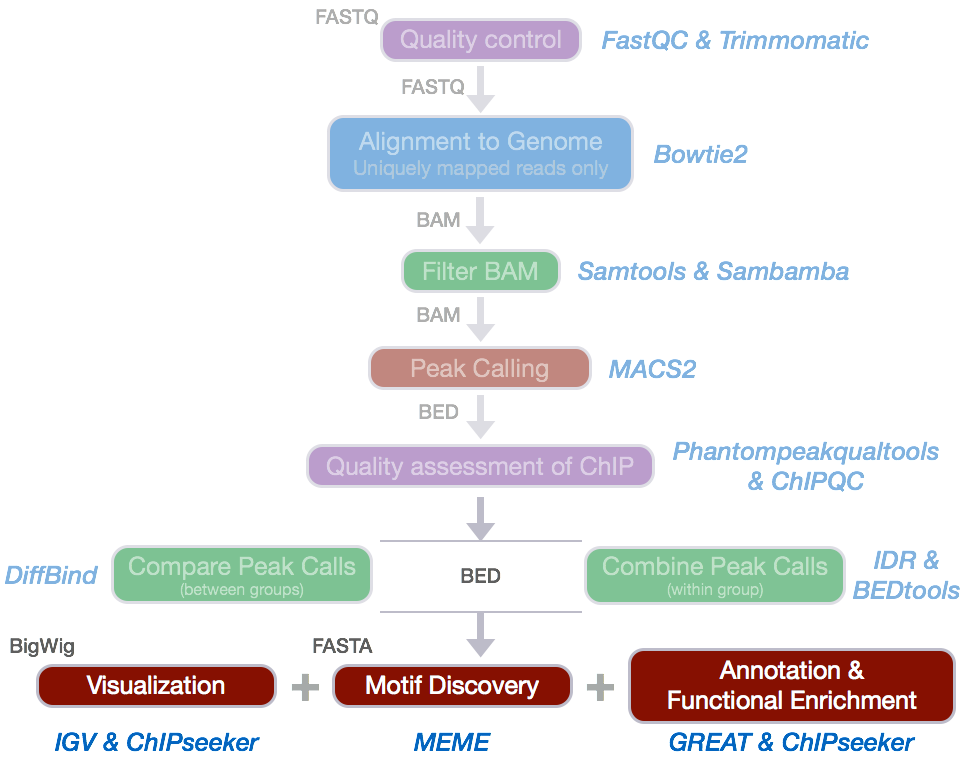
Annotation and Functional Analysis
We have identified regions of the genome that are enriched in the number of aligned reads for each of our transcription factors of interest, Nanog and Pou5f1. These enriched regions represent the likely locations of where these proteins bind to the genome. After we obtain a list of peak coordinates, it is important to study the biological implications of the protein–DNA bindings. Certain questions have always been asked: what are the genomic annotations and the functions of these peak regions?
Peak Annotation
Because many cis-regulatory elements are close to TSSs of their targets, it is common to associate each peak to its nearest gene, either upstream or downstream. ChIPseeker is an R Bioconductor package for annotating peaks. Additionally, it has various visualization functions to assess peak coverage over chromosomes and profiles of peaks binding to TSS regions.
Setting up
- Open up RStudio and open up the
chipseq-projectthat we created previously. -
Open up a new R script (‘File’ -> ‘New File’ -> ‘Rscript’), and save it as
chipseeker.RNOTE: This next section assumes you have the
ChIPseekerpackage installed for R 3.5 or higher. You will also need one additional library for gene annotation. If you haven’t done this please run the following lines of code before proceeding.BiocManager::install("ChIPseeker") - Now we can load all required libraries:
# Load libraries
library(ChIPseeker)
library(TxDb.Hsapiens.UCSC.hg19.knownGene)
library(EnsDb.Hsapiens.v75)
library(clusterProfiler)
library(AnnotationDbi)
library(org.Hs.eg.db)
Loading data
Peak annotation is generally performed on your high confidence peak calls (after looking at concordance betwee replicates). While we have a confident peak set for our data, this set is rather small and will not result in anything meaningful in our functional analyses. We have generated a set of high confidence peak calls using the full dataset. These were obtained post-IDR analysis, (i.e. concordant peaks between replicates) and are provided in BED format which is optimal input for the ChIPseeker package.
NOTE: the number of peaks in these BED files are are significantly higher than what we observed with the smaller dataset that we have been working with.
We will need to copy over the appropriate files from O2 to our laptop. You can do this using FileZilla or the scp command.
Move over the BED files from O2(/n/groups/hbctraining/chip-seq/full-dataset/idr/*.bed) to your laptop. You will want to copy these files into your chipseq-project into a new folder called data/idr-bed.
To load the data into our R session, we need to provide the names of our BED files in a list format.
# Load data
samplefiles <- list.files("data/idr-bed", pattern= ".bed", full.names=T)
samplefiles <- as.list(samplefiles)
names(samplefiles) <- c("Nanog", "Pou5f1")
Next, we need to assign annotation databases generated from UCSC to a variable:
txdb <- TxDb.Hsapiens.UCSC.hg19.knownGene
NOTE: ChIPseeker supports annotating ChIP-seq data of a wide variety of species if they have transcript annotation TxDb object available. To find out which genomes have the annotation available follow this link and scroll down to “TxDb”. Also, if you are interested in creating your own TxDb object you will find more information here.
Annotation
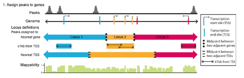
Many annotation tools use nearest gene methods for assigning a peak to a gene in which the algorithm looks for the nearest TSS to the given genomic coordinates and annotates the peak with that gene. This can be misleading as binding sites might be located between two start sites of different genes.
The annotatePeak function, as part of the ChIPseeker package, uses the nearest gene method described above but also provides parameters to specify a max distance from the TSS. For annotating genomic regions, annotatePeak will not only give the gene information but also reports detail information when genomic region is Exon or Intron. For instance, ‘Exon (uc002sbe.3/9736, exon 69 of 80)’, means that the peak overlaps with the 69th exon of the 80 exons that transcript uc002sbe.3 possess and the corresponding Entrez gene ID is 9736.
Let’s start by retrieving annotations for our Nanog and Pou5f1 peaks calls:
peakAnnoList <- lapply(samplefiles, annotatePeak, TxDb=txdb,
                       tssRegion=c(-1000, 1000), verbose=FALSE)
If you take a look at what is stored in peakAnnoList, you will see that the peak annotations have been summarized for you based on genomic features:
> peakAnnoList
$Nanog
Annotated peaks generated by ChIPseeker
11023/11035  peaks were annotated
Genomic Annotation Summary:
             Feature  Frequency
9           Promoter 17.1731833
4             5' UTR  0.2358705
3             3' UTR  0.9706976
1           1st Exon  0.5443164
7         Other Exon  1.7781003
2         1st Intron  7.2121927
8       Other Intron 28.2318788
6 Downstream (<=3kb)  0.9434818
5  Distal Intergenic 42.9102785

$Pou5f1
Annotated peaks generated by ChIPseeker
3242/3251  peaks were annotated
Genomic Annotation Summary:
             Feature  Frequency
9           Promoter  3.7939543
4             5' UTR  0.1542258
3             3' UTR  1.0795805
1           1st Exon  1.3263418
7         Other Exon  1.6347933
2         1st Intron  7.4336829
8       Other Intron 30.9685379
6 Downstream (<=3kb)  0.9561999
5  Distal Intergenic 52.6526835
ChIPseeker provides several functions to visualize the annotations using various plots. We will demonstrate a few of these using the Nanog sample. We will also show you how some of the functions can support comparing annotation information across samples.
NOTE: ChIPseeker also has functionality to generate figures for visualization (similar to what we did in
deepTools). If you are interested in testing out those functions on this data, please see the materials linked here.
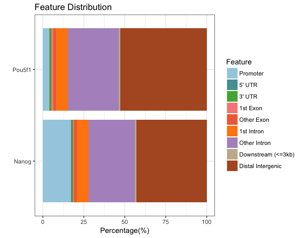
Barchart of genomic feature representation
plotAnnoBar(peakAnnoList)
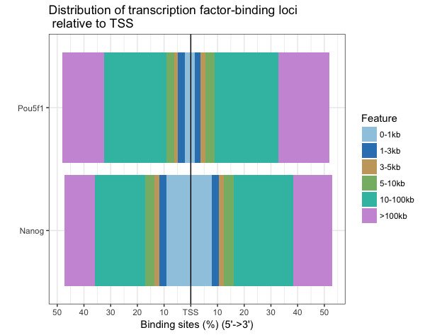
Distribution of TF-binding loci relative to TSS
plotDistToTSS(peakAnnoList, title="Distribution of transcription factor-binding loci \n relative to TSS")
Finally, it would be nice to have the annotations for each peak call written to file, as it can be useful to browse the data and subset calls of interest. The annotation information is stored in the peakAnnoList object. To retrieve it we use the following syntax:
nanog_annot <- data.frame(peakAnnoList[["Nanog"]]@anno)
Take a look at this data frame. You should see columns corresponding to your input BED file and addditional columns containing nearest gene(s), the distance from peak to the TSS of its nearest gene, genomic feature annotation of the peak and other information. Since some annotations may overlap, ChIPseeker has adopted the following priority in how it lists information:
- Promoter
- 5’ UTR
- 3’ UTR
- Exon
- Intron
- Downstream (defined as the downstream of gene end)
- Intergenic
One thing you will notice is that the gene identifiers that are listed are EntrezIDs. It would be easier to browse through the results if we had gene symbols. We will obtain this information using AnnotationDbi, an R package that provides an interface for connecting and querying various annotation databases using SQLite data storage. The AnnotationDbi packages can query the OrgDb, TxDb, EnsDb, Go.db, and BioMart annotations. There is helpful documentation available to reference when extracting data from any of these databases.
Although we have been using the TxDb database with ChIPseeker, there is limited options as to what other identifiers can be retrieved.
keytypes(TxDb.Hsapiens.UCSC.hg19.knownGene)
[1] "CDSID"    "CDSNAME"  "EXONID"   "EXONNAME" "GENEID"   "TXID"     "TXNAME"
Since we want to map our EntrezIDs to gene symbols, we will need to use another database. The EnsDb.Hsapiens.v75 database corresponds to hg19, and so is an appropriate option.
# Get the entrez IDs
entrez <- nanog_annot$geneId

# Return the gene symbol for the set of Entrez IDs
annotations_edb <- AnnotationDbi::select(EnsDb.Hsapiens.v75,
                                         keys = entrez,
                                         columns = c("GENENAME"),
                                         keytype = "ENTREZID")

# Change IDs to character type to merge
annotations_edb$ENTREZID <- as.character(annotations_edb$ENTREZID)

# Write to file
nanog_annot %>%
  left_join(annotations_edb, by=c("geneId"="ENTREZID")) %>%
  write.table(file="results/Nanog_peak_annotation.txt", sep="\t", quote=F, row.names=F)
Functional enrichment: R-based tools
Once we have obtained gene annotations for our peak calls, we can perform functional enrichment analysis to identify predominant biological themes among these genes by incorporating knowledge from biological ontologies such as Gene Ontology, KEGG and Reactome. The gene lists we have obtained through annotation can be interepreted using freely available web- and R-based tools. In this workshop we will focus on the latter, but we will also mention the former and provide resources if you are interested in web-based tools.
Over-representation analysis
There are a plethora of functional enrichment tools that perform some type of over-representation analysis by querying databases containing information about gene function and interactions. Querying these databases for gene function requires the use of a consistent vocabulary to describe gene function. One of the most widely-used vocabularies is the Gene Ontology (GO). This vocabulary was established by the Gene Ontology project, and the words in the vocabulary are referred to as GO terms.
We will be using clusterProfiler to perform over-representation analysis on GO terms associated with our list of significant genes. The tool takes as input a significant gene list and a background gene list and performs statistical enrichment analysis using hypergeometric testing. The basic arguments allow the user to select the appropriate organism and GO ontology (BP, CC, MF) to test.
Let’s start with our gene list from Nanog annotations and use them as input for a GO enrichment analysis of biological process terms.
# Run GO enrichment analysis
ego <- enrichGO(gene = entrez,
                    keyType = "ENTREZID",
                    OrgDb = org.Hs.eg.db,
                    ont = "BP",
                    pAdjustMethod = "BH",
                    qvalueCutoff = 0.05,
                    readable = TRUE)
The ego object we created contains the results of the over-representation analysis. We can extract it into a data frame and write the results to file:
# Output results from GO analysis to a table
cluster_summary <- data.frame(ego)
write.csv(cluster_summary, "results/clusterProfiler_Nanog.csv")
We can also use the ego object to visualize the results using the dotplot() function. The dotplot shows the number of genes associated with the first 50 terms (size) and the p-adjusted values for these terms (color). This plot displays the top 50 genes by gene ratio (# genes related to GO term / total number of sig genes), not p-adjusted value.
# Dotplot visualization
dotplot(ego, showCategory=50)
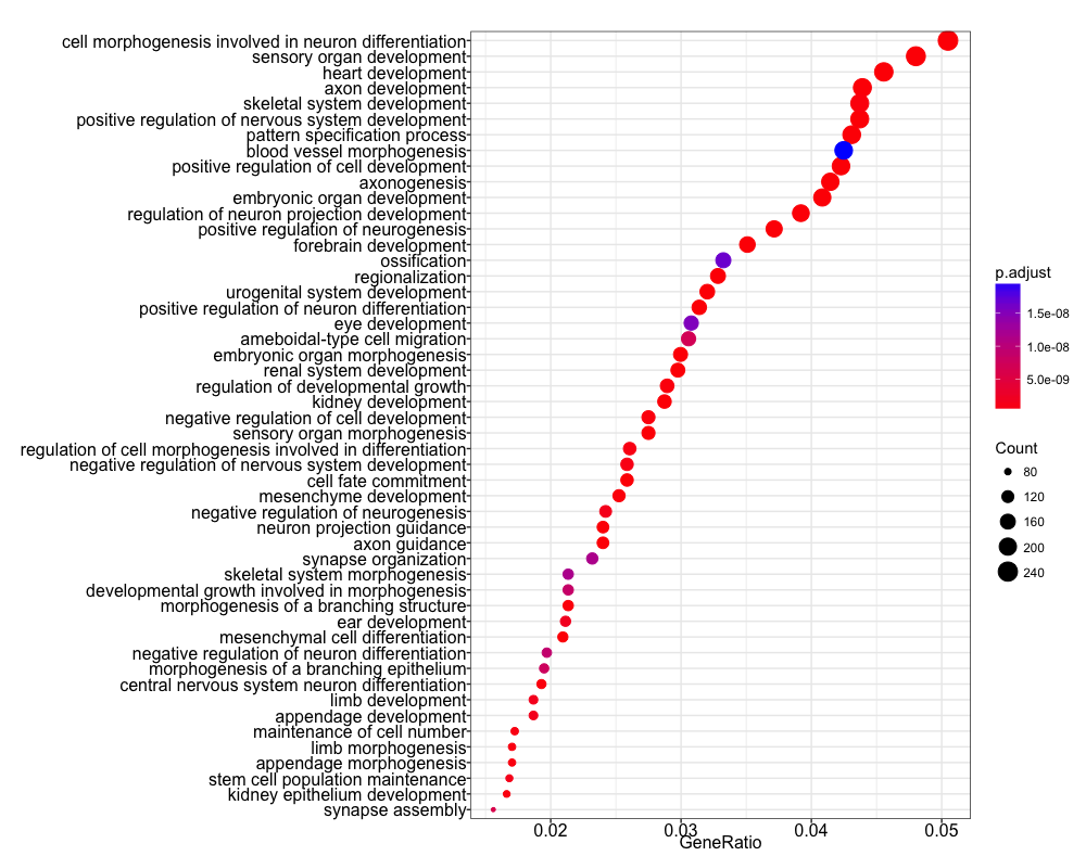
We find many terms related to development and differentiation and amongst those we see the term ‘stem cell population maintenance’. This makes sense since functionally, Nanog blocks differentiation. Thus, negative regulation of Nanog is required to promote differentiation during embryonic development. Recently, Nanog has been shown to be involved in neural stem cell differentiation which might explain the abundance of brain-related terms we observe.
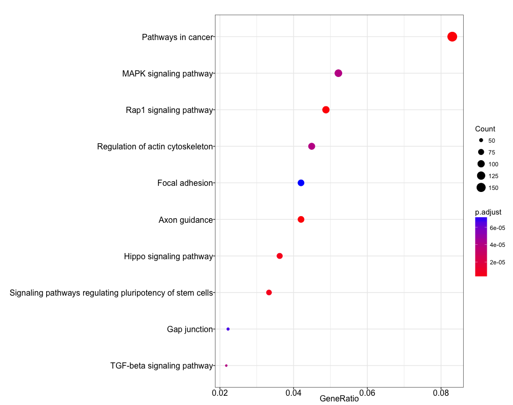
Another popular resource for pathway level annotations is the KEGG database. There is a function in clusterProfiler that allows us to perform KEGG pathway enrichment and visualize the results using the the dotplot. Again, we see a relevant pathway ‘Signaling pathways regulating pluripotency of stem cells’ is enriched.
ekegg <- enrichKEGG(gene = entrez,
                 organism = 'hsa',
                 pvalueCutoff = 0.05)

dotplot(ekegg)
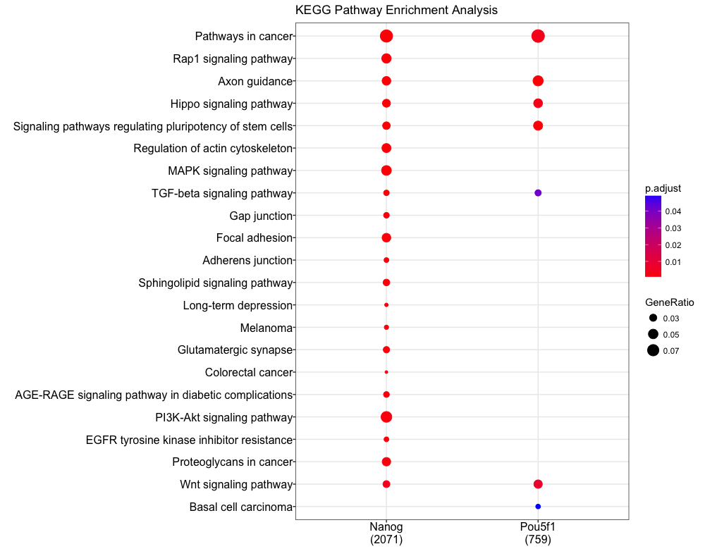
Comparing enrichment across samples
Our dataset consists of two different transcription factor peak calls, so it would be useful to be able to compare functional enrichment results side-by-side in the same plot. We can do this using the compareCluster function. We see similar terms showing up, and in particular the stem cell term is more significant (with a higher gene ratio) in the Pou5f1 target gene list.
# Create a list with genes from each sample
genes = lapply(peakAnnoList, function(i) as.data.frame(i)$geneId)

# Run KEGG analysis
compKEGG <- compareCluster(geneCluster = genes,
                         fun = "enrichKEGG",
                         organism = "human",
                         pvalueCutoff  = 0.05,
                         pAdjustMethod = "BH")
dotplot(compKEGG, showCategory = 20, title = "KEGG Pathway Enrichment Analysis")
Functional enrichment: Web-based tools
There are also web-based tool for enrichment analysis on genomic regions, and a popular one is GREAT (Genomic Regions Enrichment of Annotations Tool). GREAT is used to analyze the functional significance of cis-regulatory regions identified by localized measurements of DNA binding events across an entire genome1. It incorporates annotations from 20 different ontologies and is an easy to use tool which generates annotation and downstream functional enrichement results for genomic coordinate files. The utility of GREAT is not limited to ChIP-seq, as it could also be applied to open chromatin, localized epigenomic markers and similar functional data sets, as well as comparative genomics sets.
In the interest of time we will not go into the details of using GREAT, however we have materials linked here if you are interested in testing it out with this dataset. There also demo datasets on the GREAT website that you can use to test out the functionality of the tool.
Motif discovery
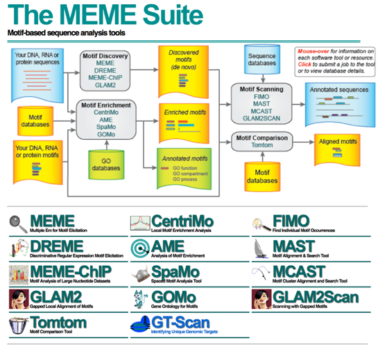
To identify over-represented motifs, we will use DREME from the MEME suite of sequence analysis tools. DREME is a motif discovery algorithm designed to find short, core DNA-binding motifs of eukaryotic transcription factors and is optimized to handle large ChIP-seq data sets.
DREME is tailored to eukaryotic data by focusing on short motifs (4 to 8 nucleotides) encompassing the DNA-binding region of most eukaryotic monomeric transcription factors. Therefore it may miss wider motifs due to binding by large transcription factor complexes.
DREME
Visit the DREME website and perform the following steps:
- You will need a FASTA file which contains the sequences of all of the genomic regions of interest. This can be generated from your IDR BED files by following the instructions in our materials linked here. In the interest of time, we have generated this file for you (using the full dataset) and it can be downloaded via this link.
- Select the downloaded
Nanog-idr-merged-dreme.fastaas input to DREME - Enter your email address so that DREME can email you once the analysis is complete
- Enter a job description so you will recognize which job has been emailed to you and then start the search
You will be shown a status page describing the inputs and the selected parameters, as well as links to the results at the top of the screen.
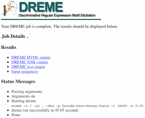
This may take some time depending on the server load and the size of the file. While you wait, take a look at the expected results.
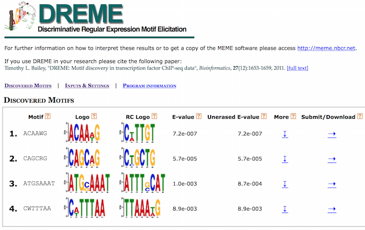
DREME’s HTML output provides a list of Discovered Motifs displayed as sequence logos (in the forward and reverse complement (RC) orientations), along with an E-value for the significance of the result.
Motifs are significantly enriched if the fraction of sequences in the input dataset matching the motif is significantly different from the fraction of sequences in the background dataset using Fisher’s Exact Test. Typically, background dataset is either similar data from a different ChIP-seq experiment or shuffled versions of the input dataset [1].
Clicking on More displays the number of times the motif was identified in the Nanog dataset (positives) versus the background dataset (negatives). The Details section displays the number of sequences matching the motif, while Enriched Matching Words displays the number of times the motif was identified in the sequences (more than one word possible per sequence).
Tomtom
To determine if the identified motifs resemble the binding motifs of known transcription factors, we can submit the motifs to Tomtom, which searches a database of known motifs to find potential matches and provides a statistical measure of motif-motif similarity. We can run the analysis individually for each motif prediction by performing the following steps:
- Click on the
Submit / Downloadbutton for motifATGYWAATin the DREME output - A dialog box will appear asking you to Select what you want to do or Select a program. Select
Tomtomand clickSubmit. This takes you to the input page. - Tomtom allows you to select the database you wish to search against. Keep the default parameters selected, but keep in mind that there are other options when performing your own analyses.
- Enter your email address and job description and start the search.
You will be shown a status page describing the inputs and the selected parameters, as well as a link to the results at the top of the screen. Clicking the link displays an output page that is continually updated until the analysis has completed. Like DREME, Tomtom will also email you the results.
The HTML output for Tomtom shows a list of possible motif matches for the DREME motif prediction generated from your Nanog regions. Clicking on the match name shows you an alignment of the predicted motif versus the match. Click here to visualize a PDF of the report
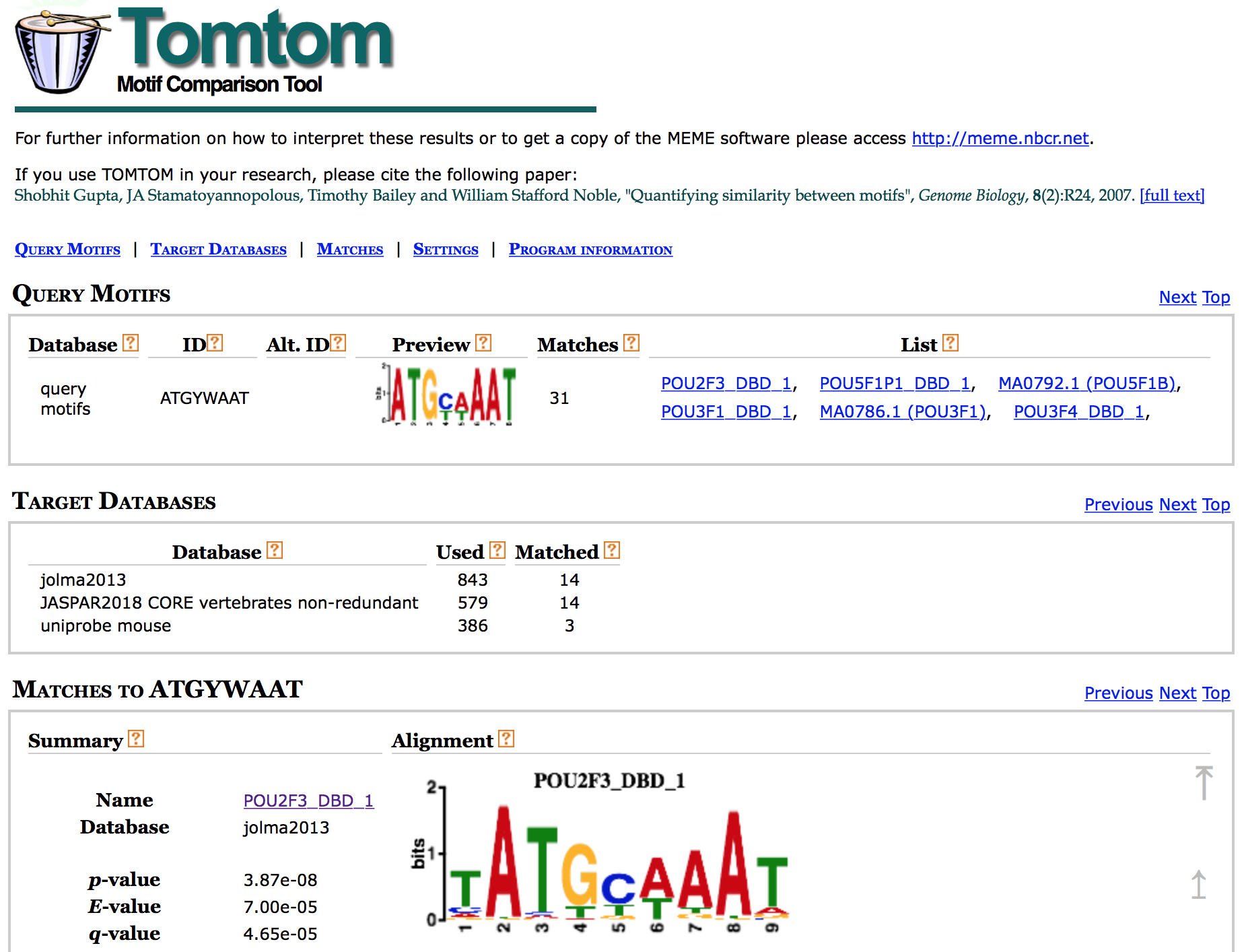
The short genomic regions identified by ChIP-seq are generally very highly enriched with binding sites of the ChIP-ed transcription factor, but Nanog is not in the databases of known motifs. The regions identified also tend to be enriched for the binding sites of other transcription factors that bind cooperatively or competitively with the ChIP-ed transcription factor.
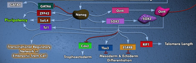
If we compare our results with what is known about our transcription factor, Nanog, we find that Sox2 and Pou5f1 (Oct4) co-regulate many of the same genes as Nanog.
 https://www.qiagen.com/us/shop/genes-and-pathways/pathway-details/?pwid=309
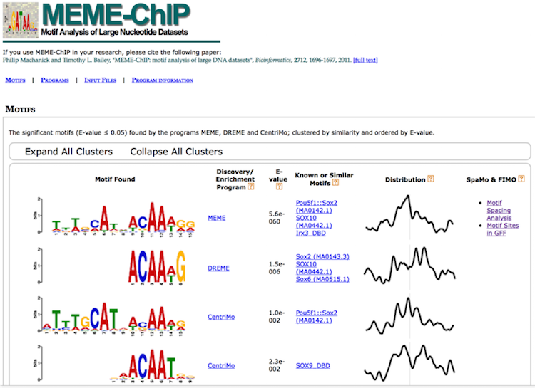
MEME-ChIP
MEME-ChIP is a tool that is part of the MEME Suite that is specifically designed for ChIP-seq analyses. MEME-ChIP performs DREME and Tomtom analysis in addition to using tools to assess which motifs are most centrally enriched (motifs should be centered in the peaks) and to combine related motifs into similarity clusters. It is able to identify longer motifs < 30bp, but takes much longer to run. The report generated by MEME-ChIP is available here.
This lesson has been developed by members of the teaching team at the Harvard Chan Bioinformatics Core (HBC). These are open access materials distributed under the terms of the Creative Commons Attribution license (CC BY 4.0), which permits unrestricted use, distribution, and reproduction in any medium, provided the original author and source are credited.