Visualization with ChIPseeker

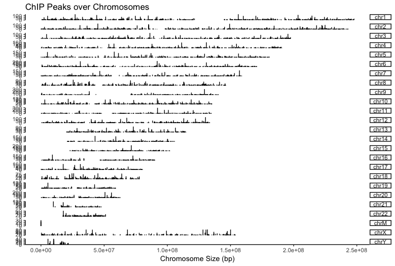
First, let’s take a look at peak locations across the genome. The covplot() function calculates coverage of peak regions across the genome and generates a figure to visualize this across chromosomes. We do this for the Nanog peaks and find a considerable number of peaks on all chromosomes.

# Assign peak data to variables
nanog <- readPeakFile(samplefiles[[1]])
pou5f1 <- readPeakFile(samplefiles[[2]])

# Plot covplot
covplot(nanog, weightCol="V5")

NOTE: In the covplot() function we provide the column which represents the amount of enrichment (weightCol="V5"), and that is the value plotted on the y-axis. This is usually some score value; in our case this is the IDR score.

Using a window of +/- 1000bp around the TSS of genes we can plot the density of read count frequency to see where binding is relative to the TSS or each sample.

# Prepare the promotor regions
promoter <- getPromoters(TxDb=txdb, upstream=1000, downstream=1000)

# Calculate the tag matrix
tagMatrixList <- lapply(as.list(samplefiles), getTagMatrix, windows=promoter)

## Profile plots
plotAvgProf(tagMatrixList, xlim=c(-1000, 1000), conf=0.95,resample=500, facet="row")

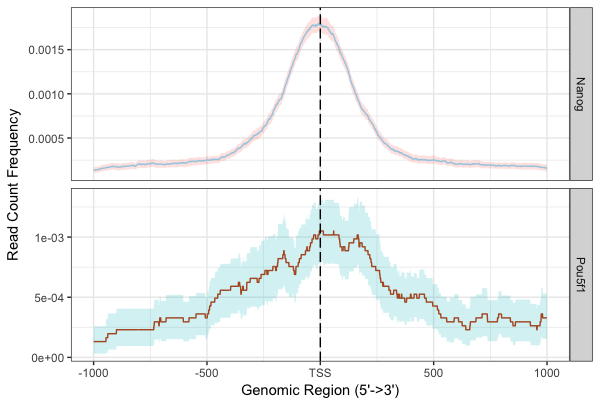
With these plots the confidence interval is estimated by bootstrap method (500 iterations) and is shown in the grey shading that follows each curve. The Nanog peaks exhibit a nice narrow peak at the TSS with small confidence intervals, whereas the Pou5f1 peaks display a bit wider and less smoothed peak around the TSS with larger confidence intervals.

The heatmap is another method of visualizing the read count frequency relative to the TSS.

# Plot heatmap
tagHeatmap(tagMatrixList, xlim=c(-1000, 1000), color=NULL)

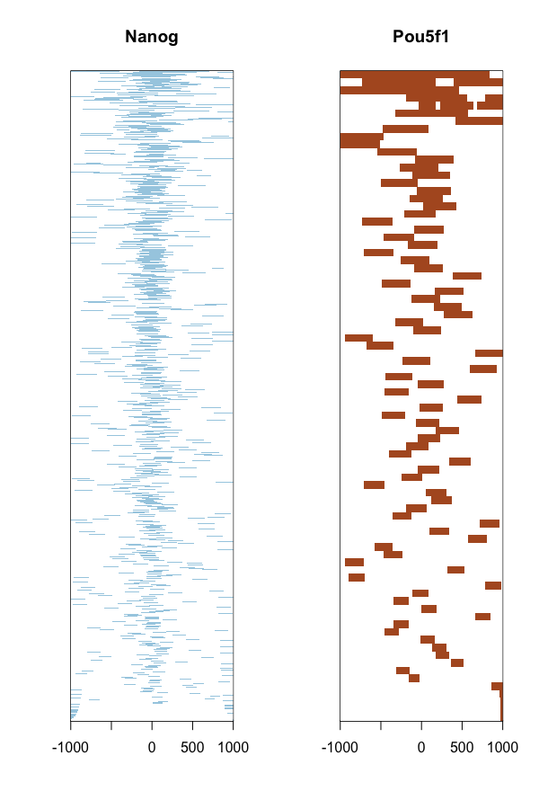
NOTE: The profile plots and heatmaps are similar to what we did using deepTools in the visualization lesson, however here the amplitude of the peak is based on the number of peaks and not on the number of reads aligning (since BAM files are not involved). ChIPseeker is useful for getting a quick look at your data, but for increased accuracy and flexibility in customizing your figure we recommend the deepTools methods.

---

This lesson has been developed by members of the teaching team at the Harvard Chan Bioinformatics Core (HBC). These are open access materials distributed under the terms of the Creative Commons Attribution license (CC BY 4.0), which permits unrestricted use, distribution, and reproduction in any medium, provided the original author and source are credited.