Learning Objectives
- Open VCF files in IGV
- Load additional tracks in IGV
- Perform basic tasks in IGV, such as renaming tracks, resizing tracks and navigating to different regions
- Saving an IGV session and opening a saved IGV session
Downloading our VCF file with FileZilla
The first thing we need to do to visualize our variants in IGV is to download our VCF to our local computer from the O2 cluster using FileZilla. Below is a refresher on the steps that we need to do in order to connect to O2 using FileZilla.
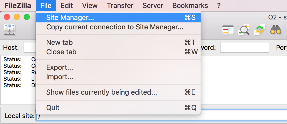
Filezilla - Step 1
Open up FileZilla, and click on the File tab. Choose ‘Site Manager’.
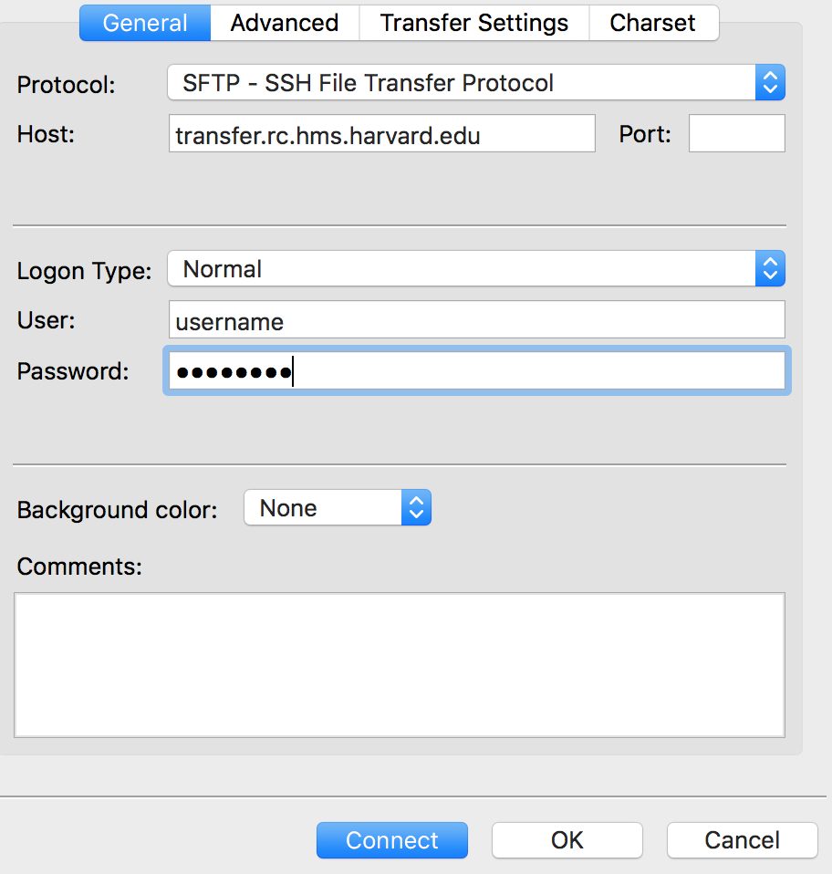
Filezilla - Step 2
Within the ‘Site Manager’ window, do the following:
- Click on ‘New Site’, and name it something intuitive (e.g. O2)
- Host: transfer.rc.hms.harvard.edu
- Protocol: SFTP - SSH File Transfer Protocol
- Logon Type: Normal
- User: Username (i.e., rc_trainingXX)
- Password: O2 password
- Click ‘Connect’
NOTE: While using the temporary training accounts on the O2 cluster, two-factor authentication IS NOT required. However, if you explore this lesson when using your personal account, two-factor authentication IS required.
In order to connect your computer using
FileZillato the O2 cluster, follow steps 1-7 as outlined above. Once you have clicked ‘Connect’, you will receive a Duo push notification (but no indication in Filezilla) which you must approve within the short time window. Following Duo approval,FileZillawill connect to the O2 cluster.
Transferring the VCF file
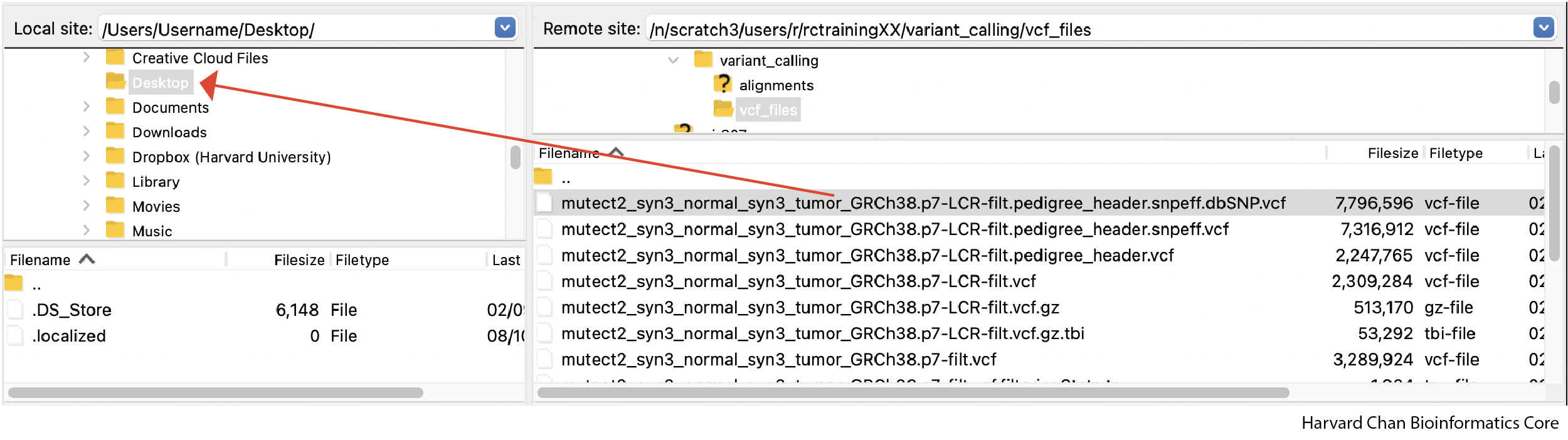
Once you are connected to O2, navigate the O2 window to where your VCF files are stored:
/n/scratch/users/r/rc_trainingXX/variant_calling/vcf_files
From here you should see your annotated VCF file:
mutect2_syn3_normal_syn3_tumor_GRCh38.p7-pass-filt-LCR.pedigree_header.snpeff.dbSNP.vcf
Drag this file over to your computer and place it in the appropriate directory. We are going to place ours in Desktop.
NOTE: If you do this transfer on your own O2 account, it will have two-factor authentication and you will need approve a Duo push notification before the download starts.
Viewing Variants in IGV
Integrative Genomics Viewer (IGV) is an application developed by the Broad Institute that we can use to visualize a wide variety of genomics tracks, including:
- BAM/SAM files
- BED files
- BEDGraph files
- VCF files
- Wiggle files
- BigWig files
- Many more
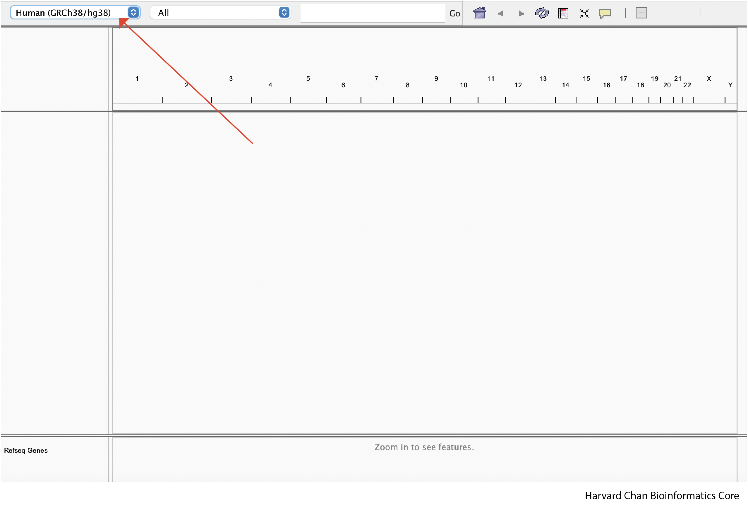
Selecting a Genome
To get started, we are going to open up IGV on our computers. Once open, we are going to navigate to the reference genome that we are interested in using from the dropdown menu in the top left of the IGV window. In this case, we are going to select “Human(GRCh38/hg38)”:
Loading Our VCF File
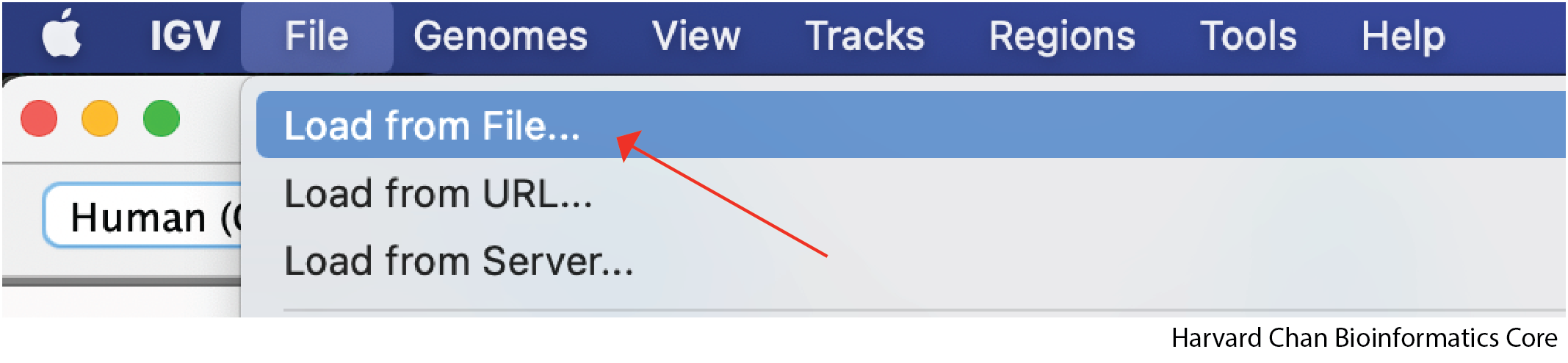
In order to load a file, like our VCF file, into IGV, we need to go to the top of our screen and left-click File → Load from File...:
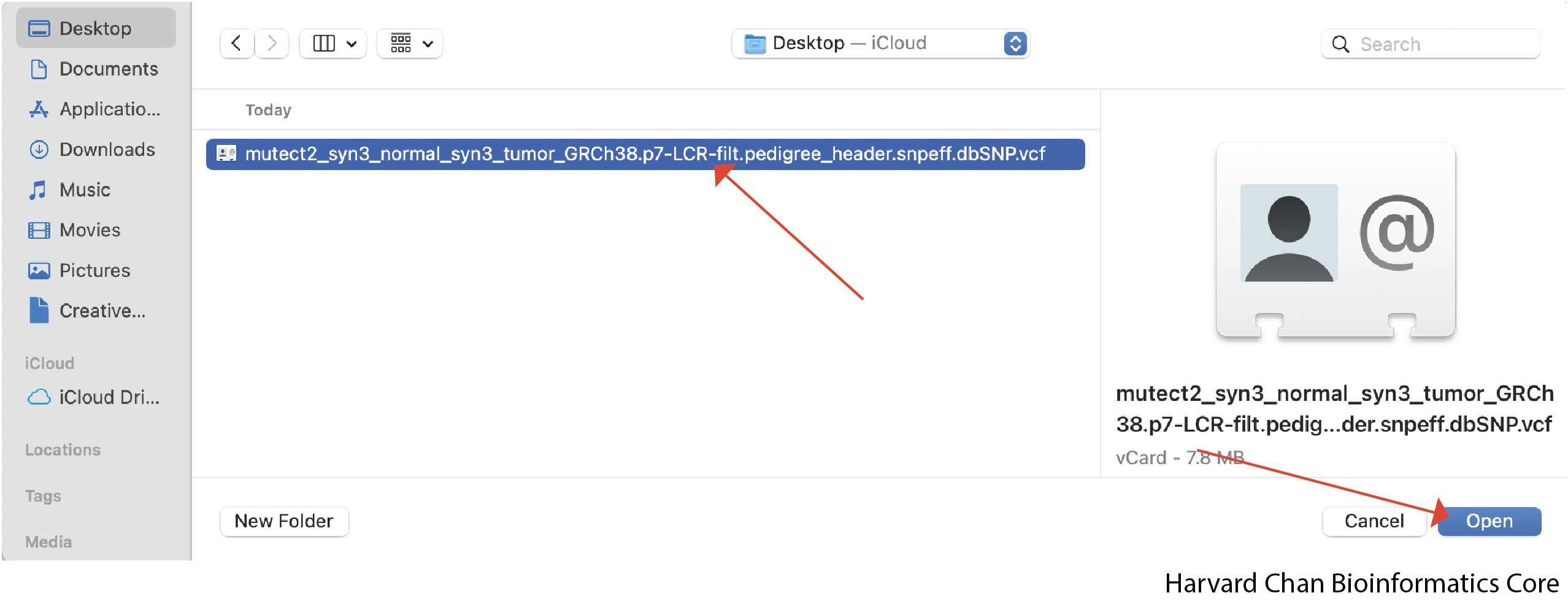
Then select the file we wish to open and left-click Open:
Now our IGV window should display the loaded file:
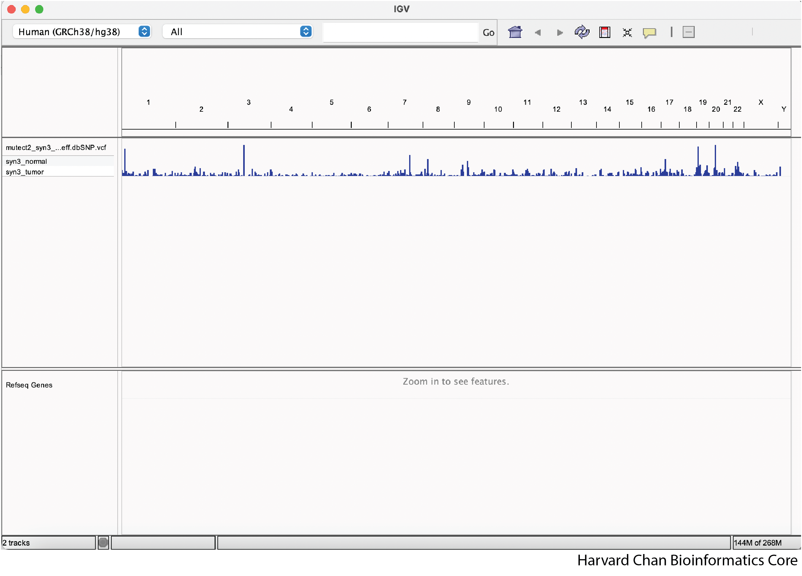
This loaded file is referred to as a track in IGV. We can have multiple tracks loaded as once and in the next section we will demonstrate how to load tracks provided by IGV.
Load IGV Provided Tracks
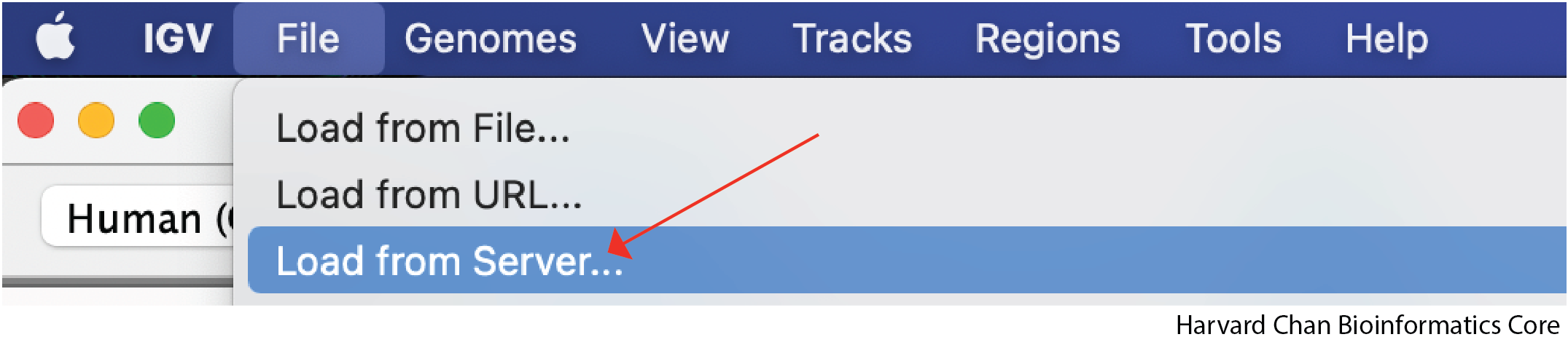
For a select few genomes, like human, IGV comes with a few annotation tracks such as RefSeq genes. While Refseq genes is loaded by default in the lower panel of the IGV window, the other tracks are not automatically loaded. Let’s see how to load these track by left-clicking on File → Load from Server...:
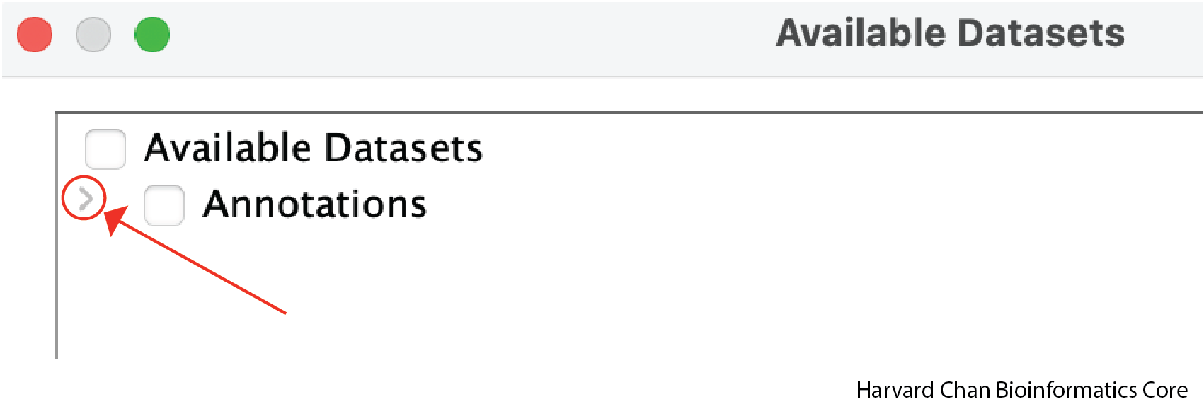
Left-click the dropdown arrow on the left side of the window to expand all of the possible provided annotation tracks:
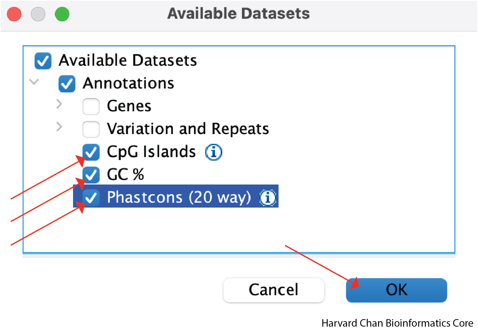
Select the checkboxes next to CpG Islands, GC % and Phastcons (20 way) and left-click Ok:
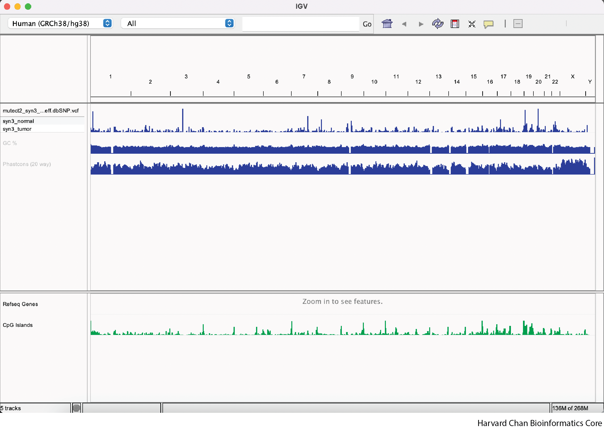
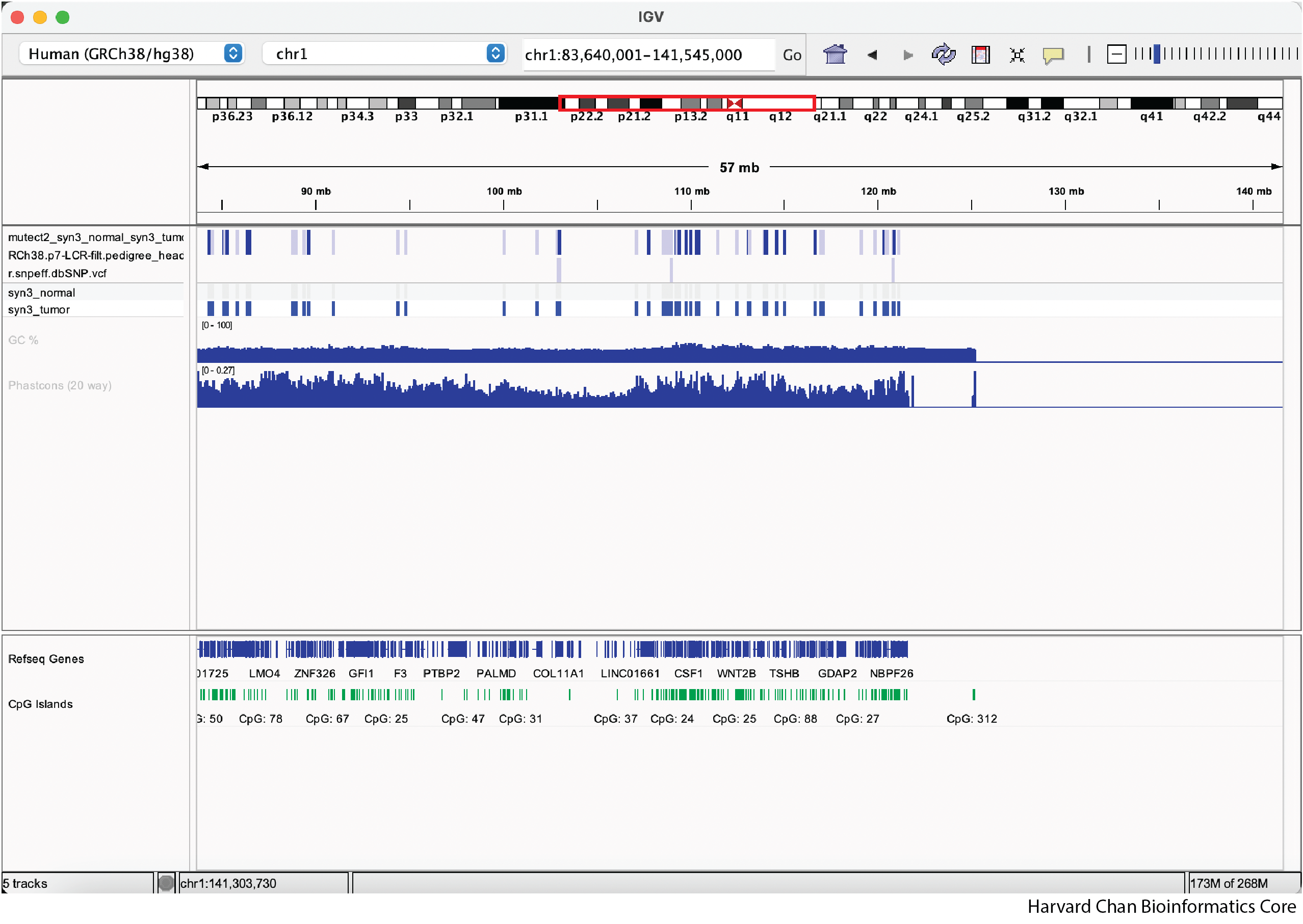
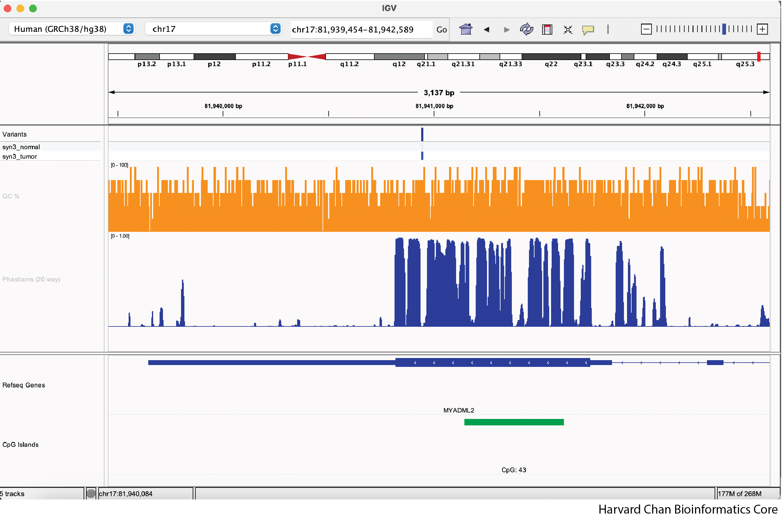
Now our IGV window should have additional tracks and look like:
Navigating IGV
Now that we have our tracks of interest loaded, we likely want to navigate around them to view our variants.
Zooming in/out on Regions
The first way that we can zoom in on a region in IGV is to left-click and hold while dragging over the region we are interested in. This can be iteratively done as one narrows down the region that they are interested in viewing.
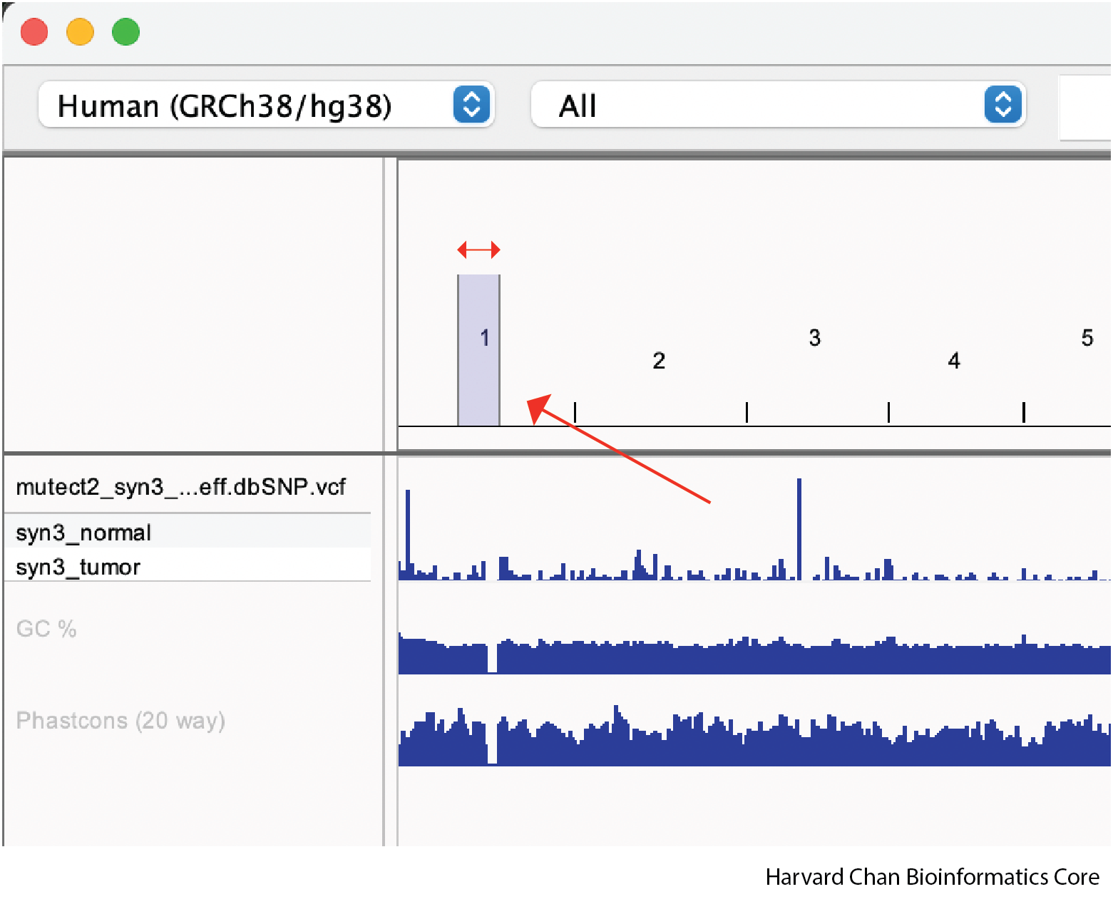
Once we zoom, our IGV window might look like:
We can zoom out and in using the - and +, respectively, on the right of the top bar:
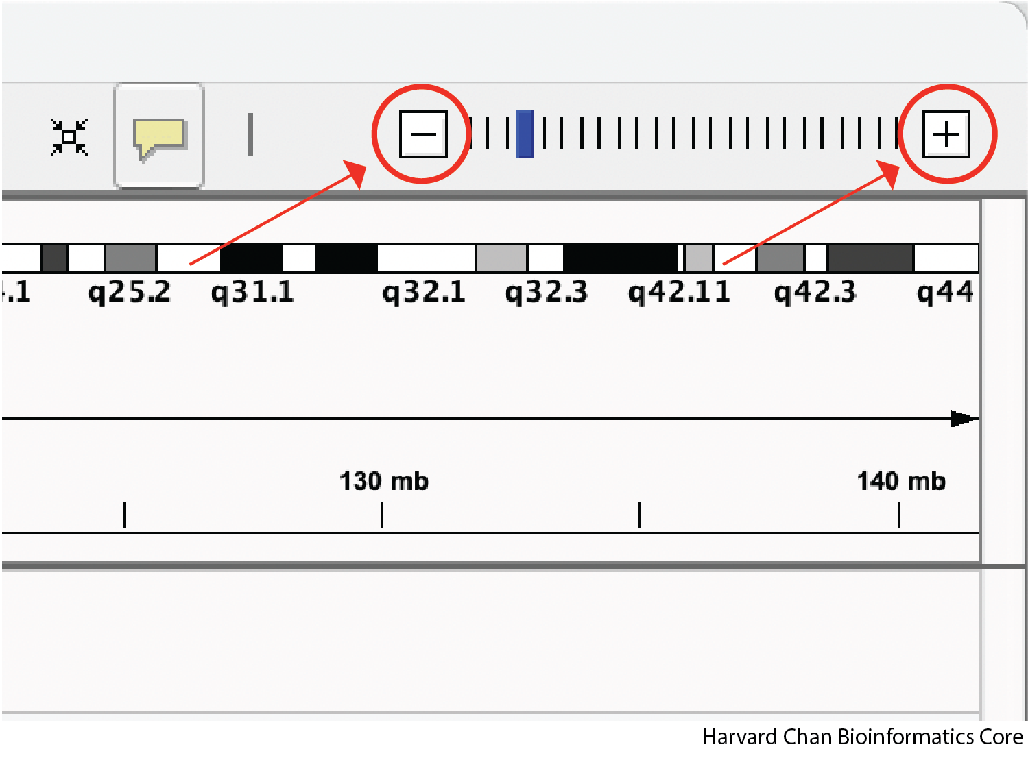
NOTE: If you can’t see the - and/or + sign on the right side of the screen, you may need to widen your window. You can see in our image above this one that we couldn’t see the + sign, but we made the IGV window wider and then we could see it.
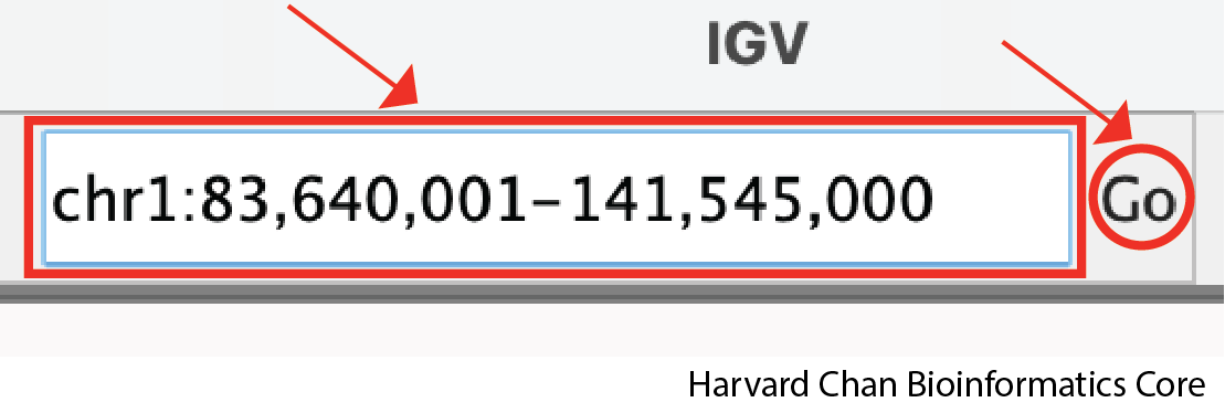
Jumping to Regions
We can jump to a given region in the genome using the following syntax in the middle of the top bar:
chr<Chromosome_Number>:<Start_position>:<End_position>
Then left-clicking Go.
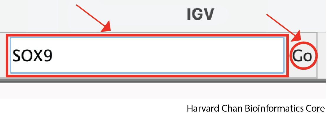
Alternatively, if there is a gene we are particularly interested in going to, we can also enter the gene’s name in this same box and left-click Go:
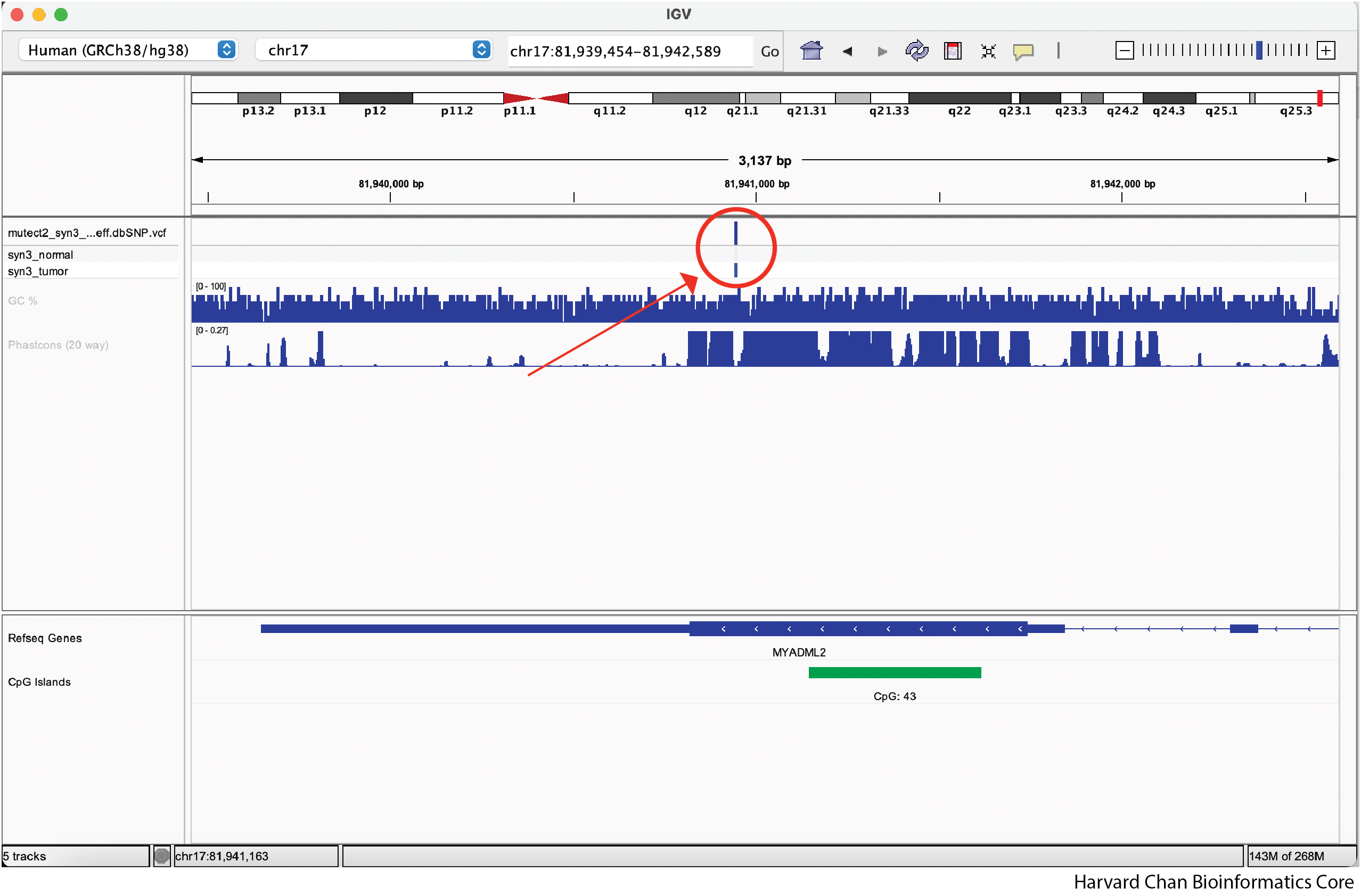
If we zoom in enough we can get down to seeing individual variants. Underneath the top part of the variant track, we can see the tracks for the variant in the normal and tumor samples.
Modifying Tracks
Now that we have an idea of how we can navigate in the IGV window, we want to learn how to modify the tracks. IGV provides lots of ways in which you can modify the tracks.
Resizing Tracks
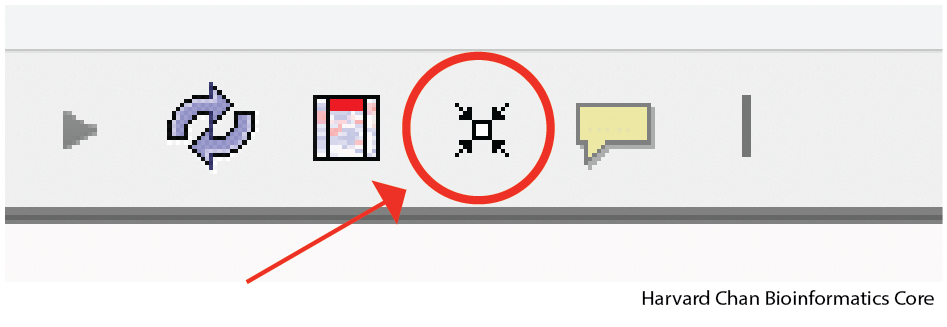
First, we might want to be interested in resizing the tracks. Currently, we have a lot of whitespace that we might want to eliminate. The easiest way eliminate lots of this whitespace is to hit the button on the top bar to “Resize tracks to fit in window”:
Now the tracks should fit into the window space a bit better and look like:
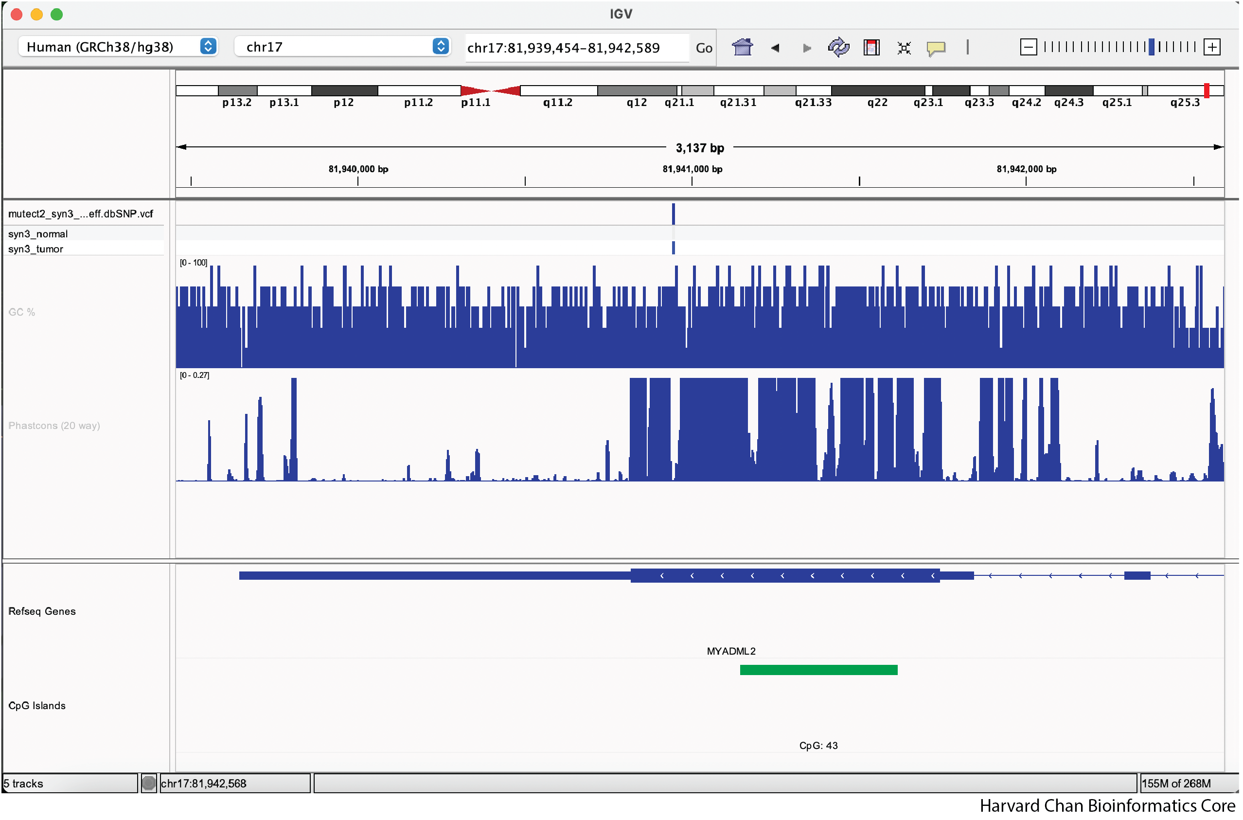
NOTE: If you have too few tracks, like we have here, they likely won’t encompass all of the white space or if you have too many tracks, IGV might not be able to cram them all into the window and you will have a scroll bar on the side.
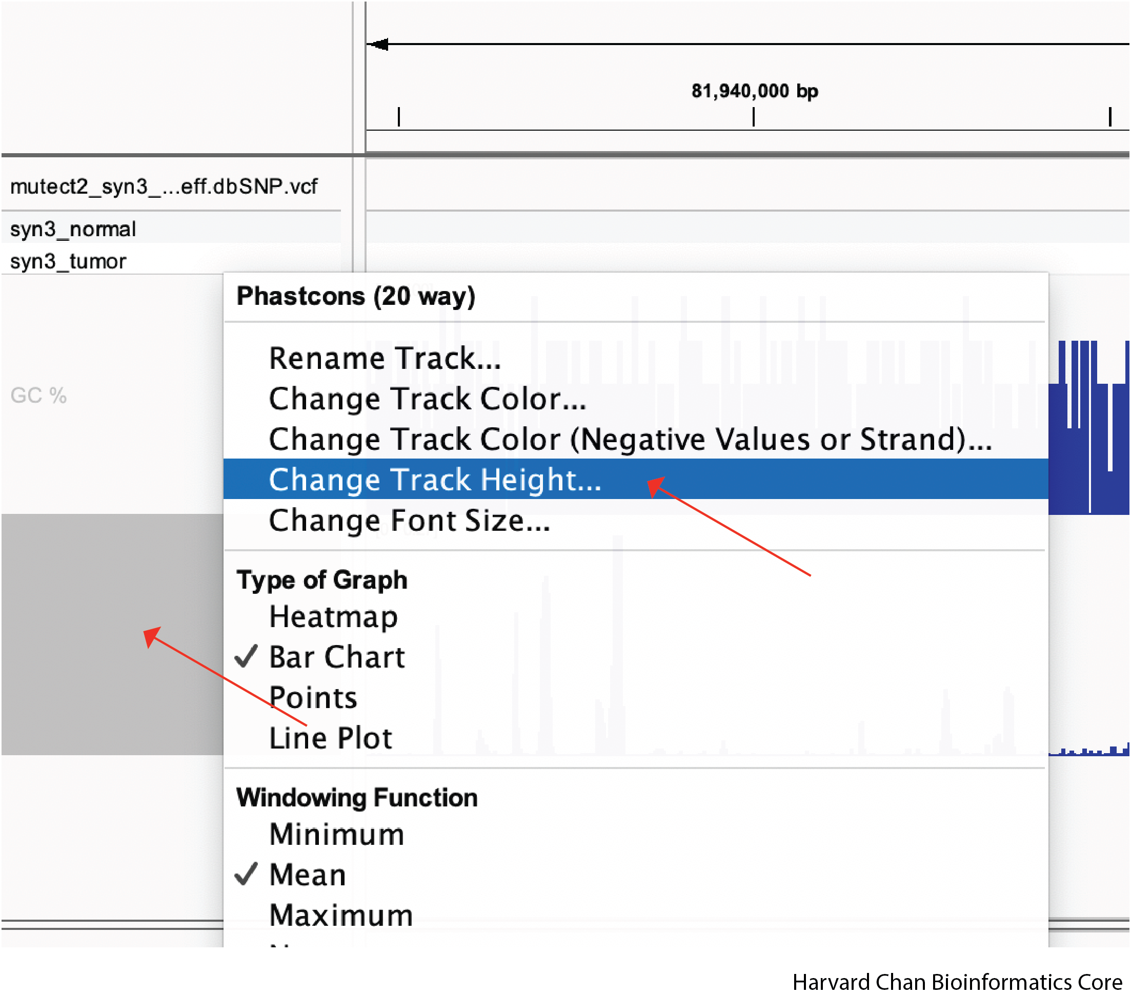
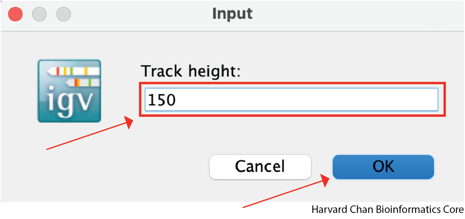
We can also manually adjust the track height by right-clicking on the track that we want to alter in size and the left-clicking “Change Track Height..”
A window should pop-up and allow you to modify the height. Once you have selected a height you can left-click OK and the track will be resized.
Modifying Track Data Range
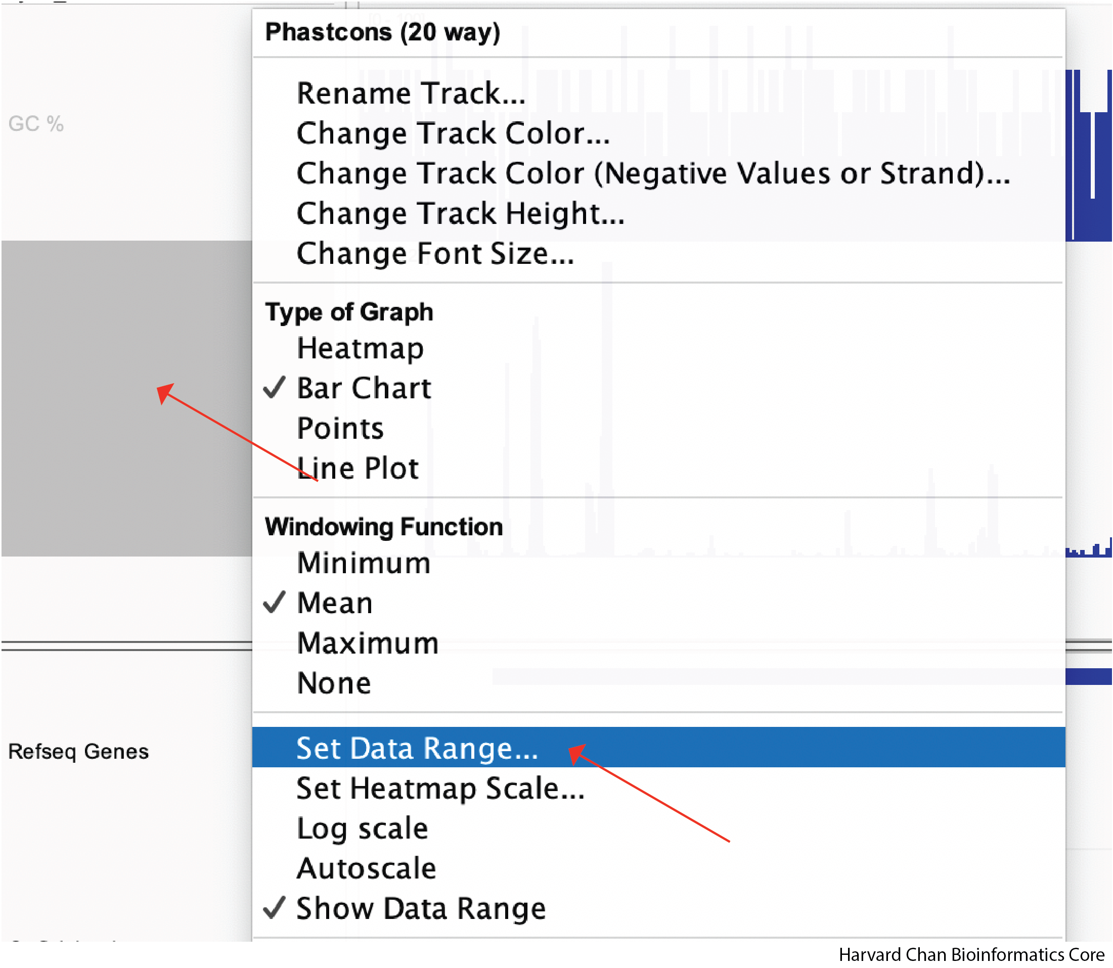
We can also adjust the data range that we want displayed in the track. Similarly to resizing the track height, we start by right-clicking the track we want to adjust, but this time we will left-click “Set Data Range…”
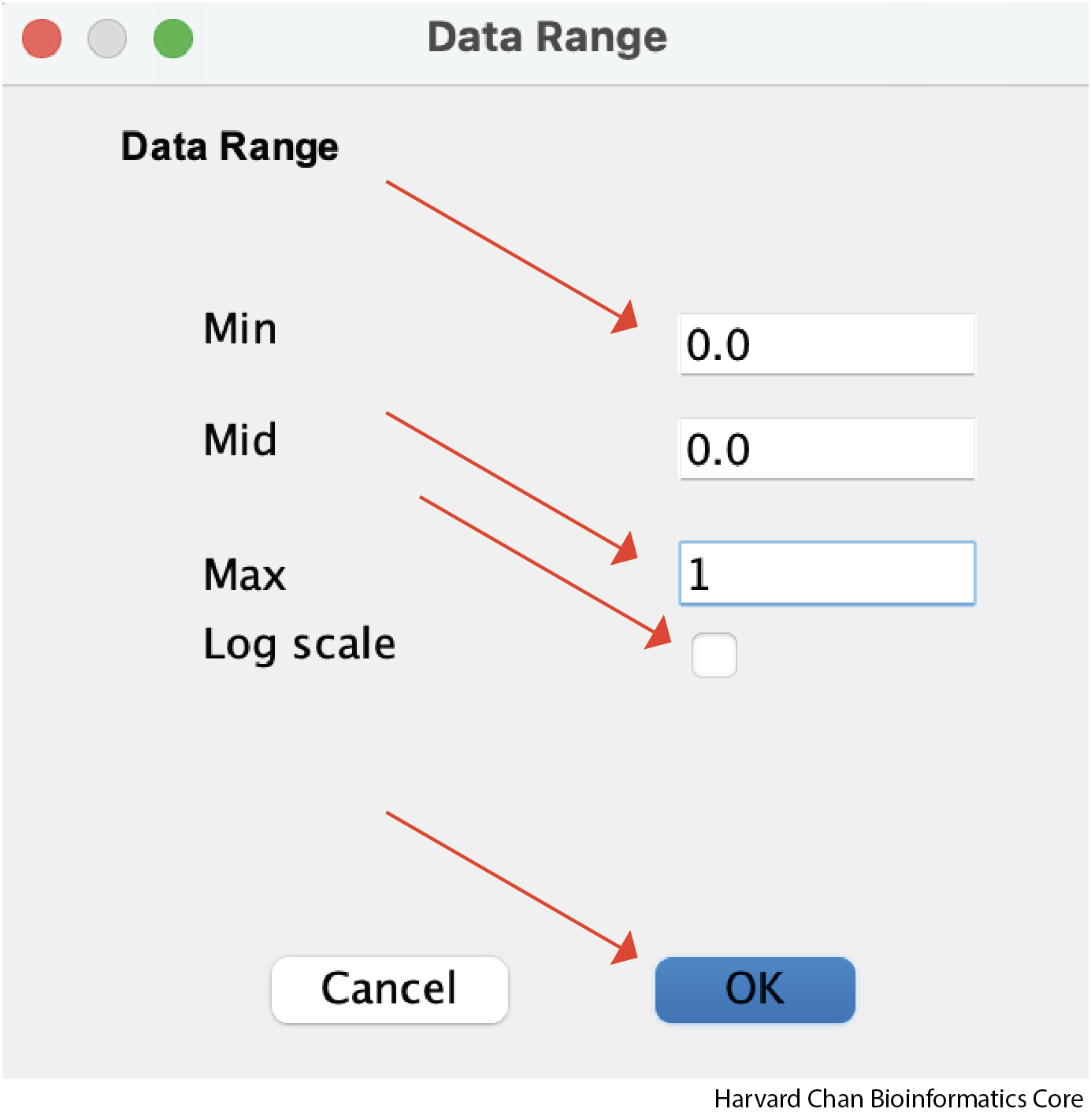
A window should pop-up and allow you to select the minimum, maximum and whether you would like the data to be log-scaled. Once you have selected the parameters you want, you can left-click OK:
Renaming Tracks
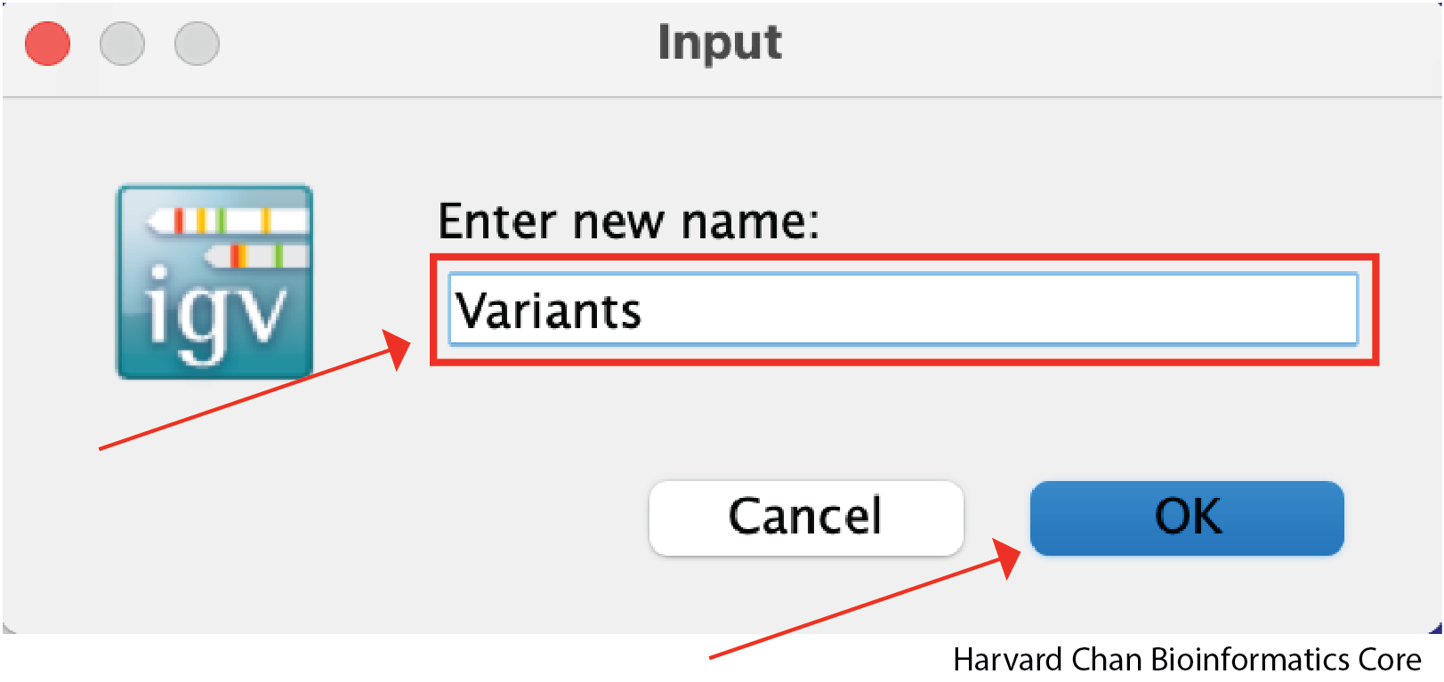
When tracks are loaded from files, they are named by the filename and sometimes these names can be long and unwieldy within IGV. Therefore, we are oftentimes interested in changing the track name to something that is more easy to understand. To change the track name, we need to right-click on the track and then left-click “Rename Track…”:
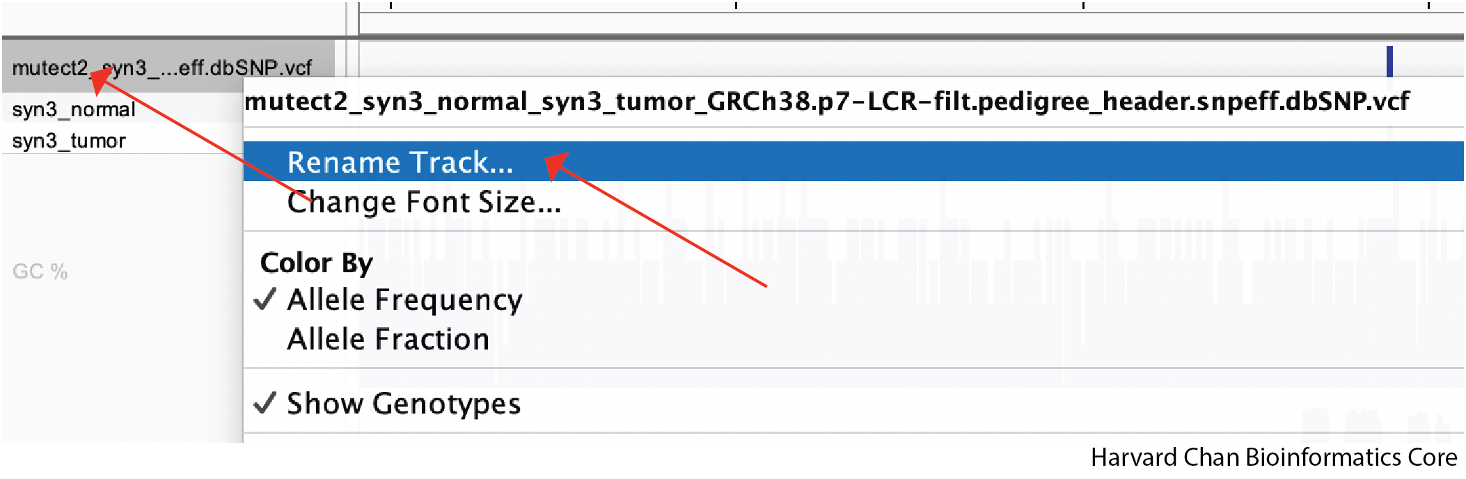
A window should pop-up and allow you to type the desired name of the track. Once you have typed the desired name, left-click OK:
Changing Track Color
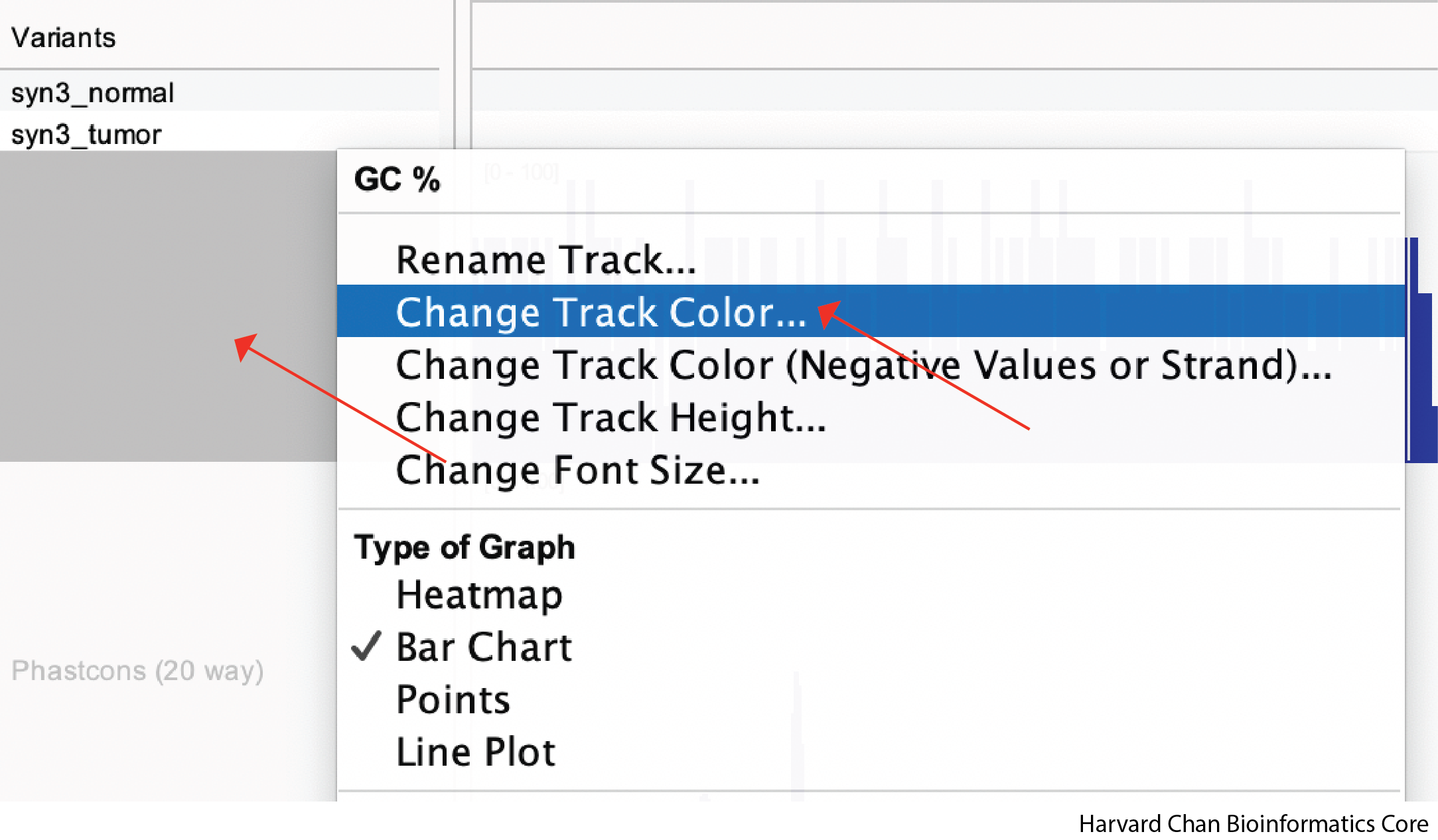
Many tracks load into IGV as blue by default, but you do have options for which color you’d like the tracks to be. In order to change the color of a track, right click on the track and left-click “Change Track Color…”:
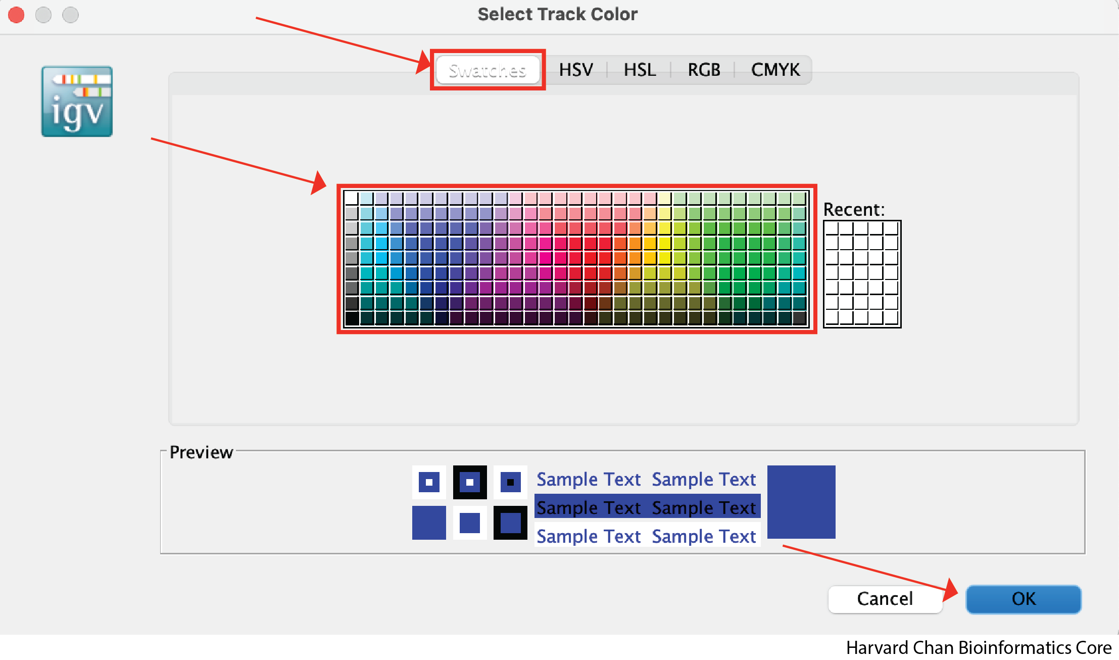
A window will pop-up on the default “Swatches” tab on the top. You can pick from a wide array for pre-selected colors here. If you find one you like, left-click the color then click OK:
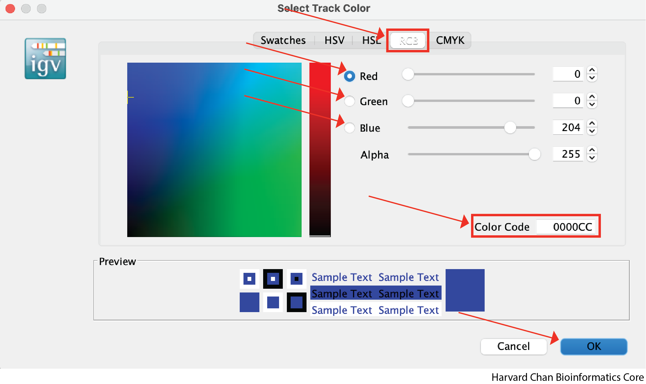
However, you may want finer control over your color selection and you can use some of the other tabs to do this. The “RGB” tab allows you to define the level of red, green and blue you want in the color. Of particular note, it also allows you to place the hexidemical code for the color you want in the “Color Code” text box. For instance, this could be of interest if you are trying to keep consistent colors from other figures where you defined a hexidecimal code for a given dataset. Once you have selected a color that you like, you can left-click OK:
Now that we’ve changed a few features in our IGV window it should now look something like this:
Changing Type of Graph
Different types of data might be visualized better in different formats. For example, we might think that “GC %” is better visualized as a line rather than as a barplot. In order to change this barplot to a line plot, we need to right-click on the track and then left-click on “Line Plot”:
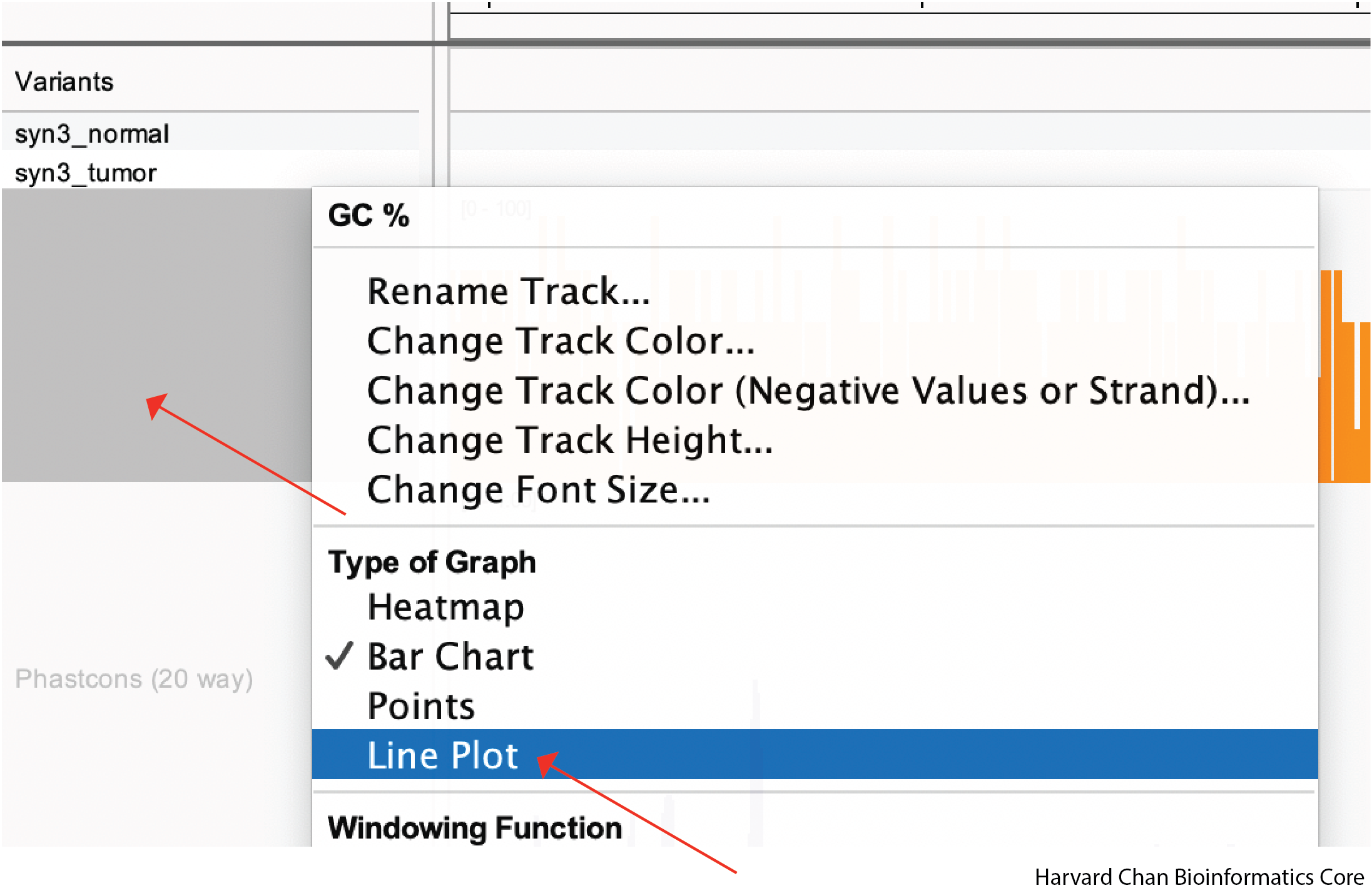
Depending on your datatype, different types of plots might be more appropriate than others.
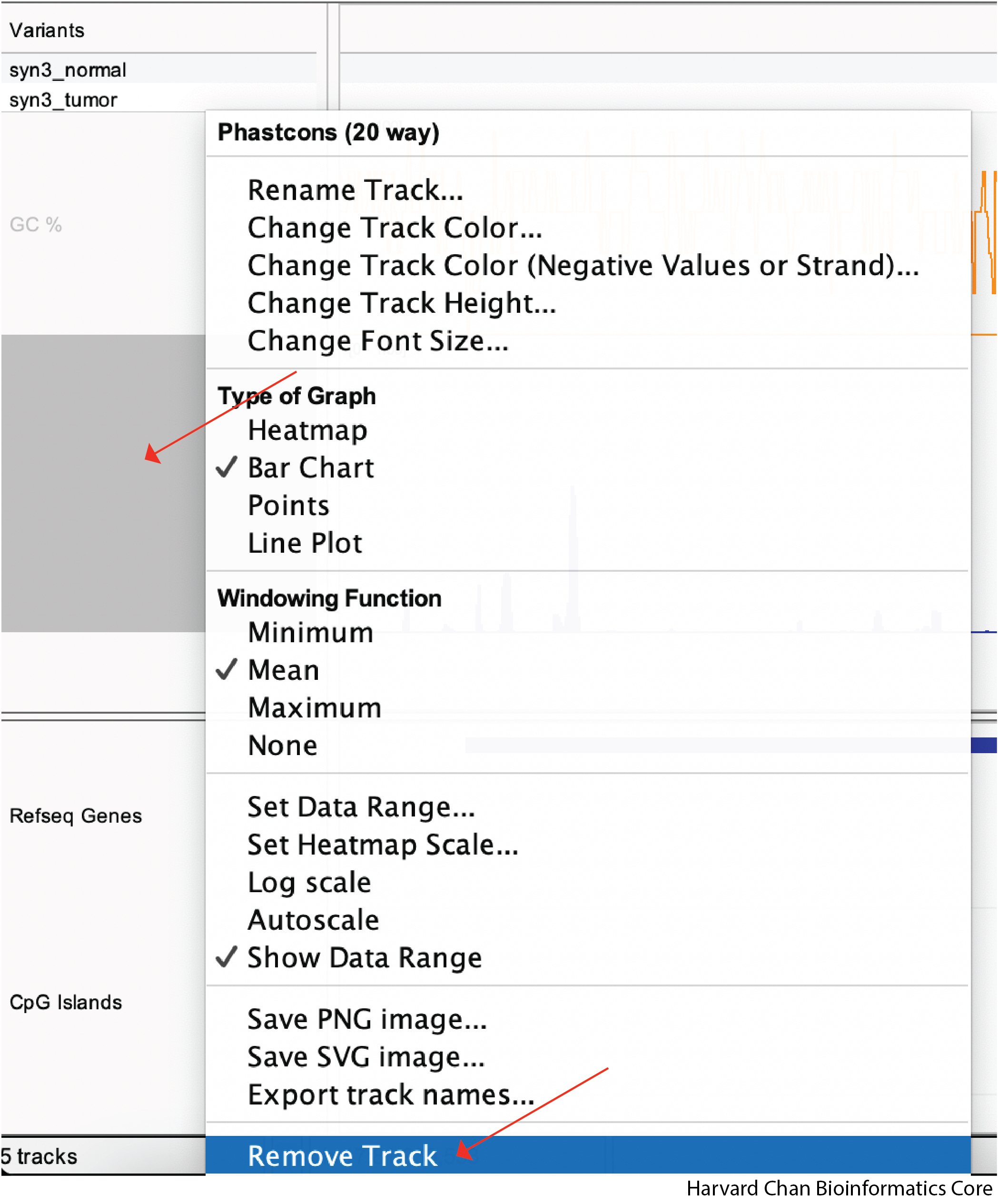
Remove Track
Lastly, you may want to remove a track from your IGV window. In order to remove a track, right-click on the track and then left-click on “Remove Track”:
Saving and Loading IGV Sessions
Oftentimes, you’ll want to save your IGV session or load up an IGV session that you’ve been previously working on. Below we will describe how to save and load IGV sessions.
Saving an IGV Session
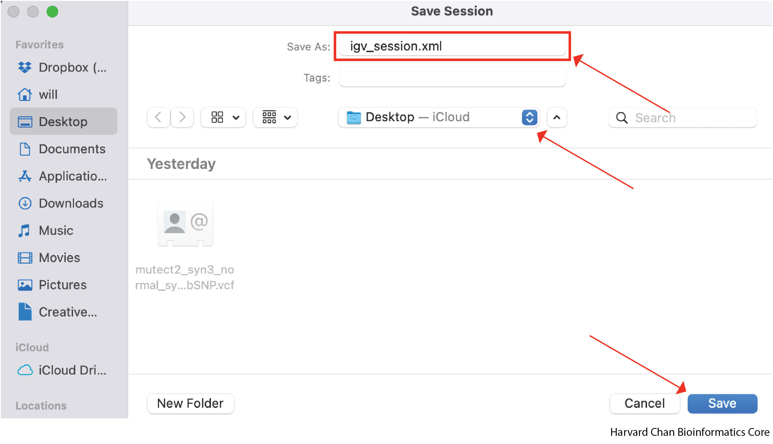
Now that you have edited your tracks to get them just the way you want you them, you might want to save the IGV session so that you can easily reload it for when you want to revisit it. To save your IGV session, go to the top bar and left-click File → Save Session...:
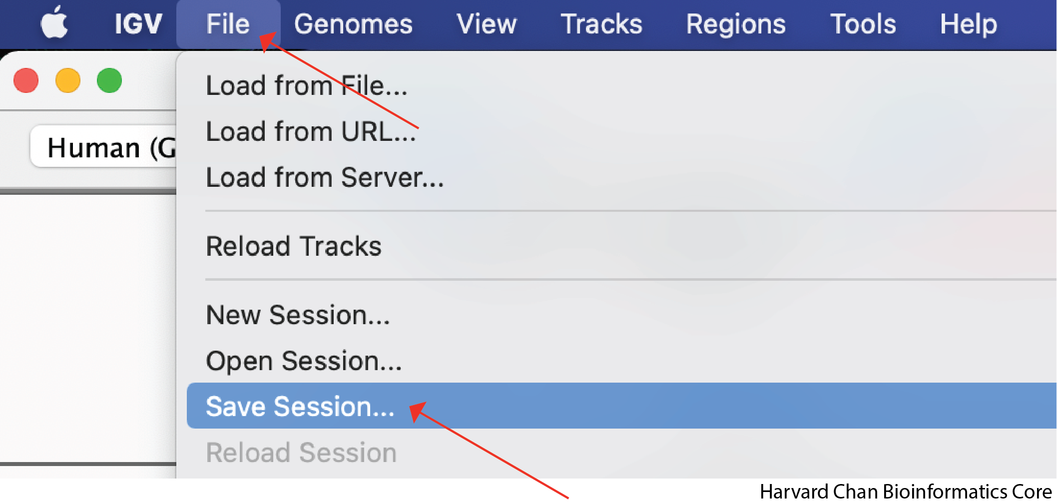
Select a name and location for the IGV session to be saved under and left-click Save. It will then be saved as an XML file.
Let’s go ahead and close our IGV session now.
Loading an IGV Session
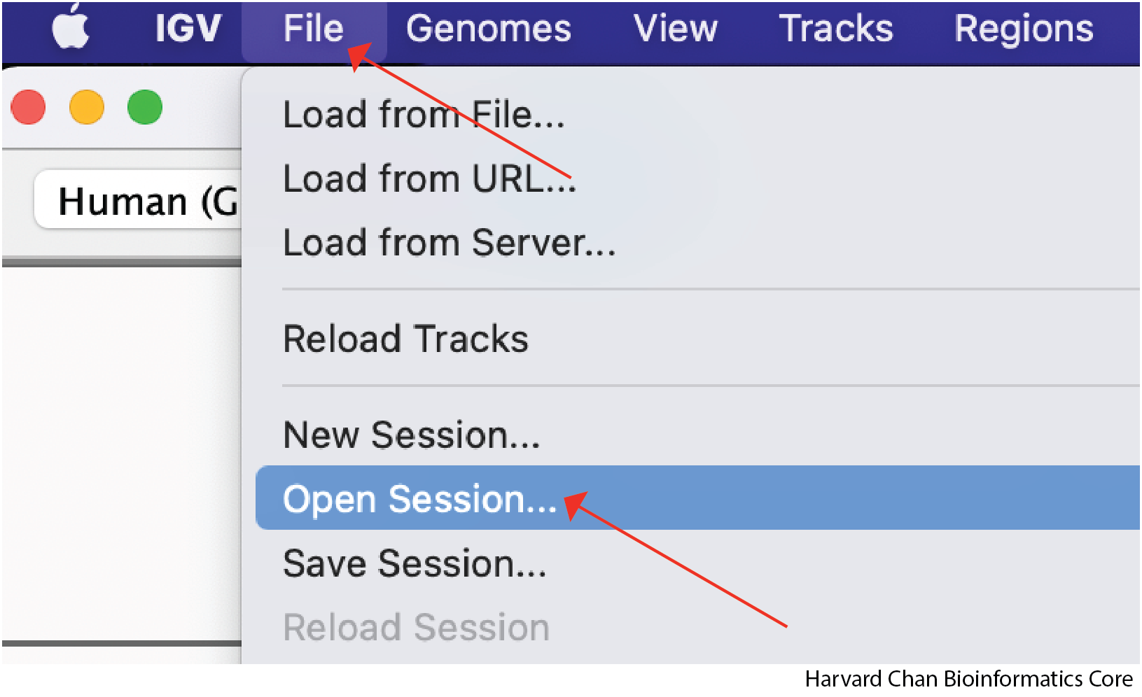
If we now open IGV back up, we will notice that it provides a fresh session. If we want to load a previous IGV session we will need to load it. To load an IGV session, go to the top bar and left-click File → Open Session...:
A window should pop-up and let you select the file you would like to load. Left-click the file you would like to load and then left-click Open:
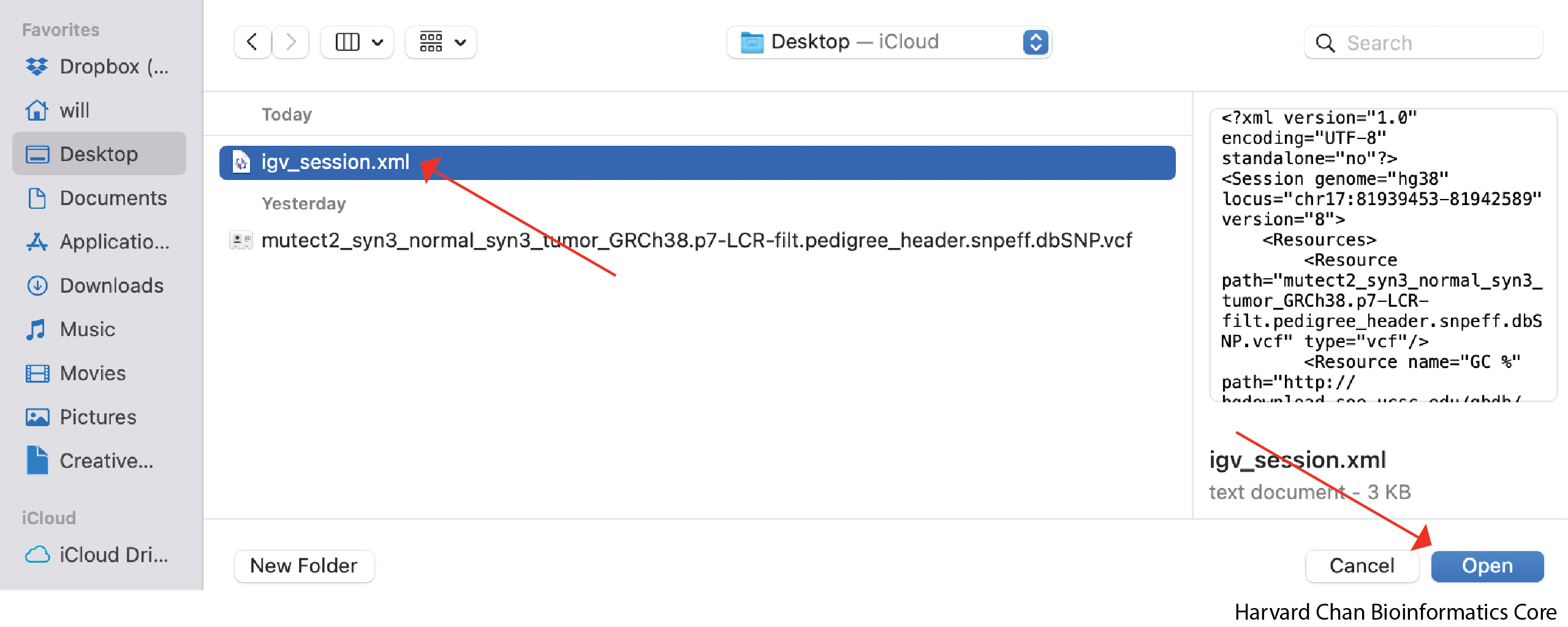
We can now see that we have loaded our previous IGV session! It is VERY IMPORTANT that if you move files that were loaded into IGV into a different location on your computer, IGV will not be able to find them and therefore not load your saved session!
Exercises
1) Download and load the SnpSift file that we created with “High Impact” mutations
2) Load the IGV provided “Variation and Repeats” track to your IGV session
3) Change the height of the CpG Islands track to 60
4) Navigate to your favorite gene. Do you see any high-impact variants there?
5) Find a high impact variant on Chromosome 4
6) Rename the “Refseq Genes” track to “Genes”
7) Save the IGV session as “Improved_IGV_session.xml”
8) Bonus Challenge Change the type of plot for “GC%” from a line plot to a heatmap.
This lesson has been developed by members of the teaching team at the Harvard Chan Bioinformatics Core (HBC). These are open access materials distributed under the terms of the Creative Commons Attribution license (CC BY 4.0), which permits unrestricted use, distribution, and reproduction in any medium, provided the original author and source are credited.