Approximate time: 90 minutes
Learning Objectives:
- Understand the theory of integration with CCA
Single-cell RNA-seq clustering analysis: Integration theory
Goals:
- To align same cell types across conditions.
Challenges:
- Aligning cells of similar cell types so that we do not have clustering downstream due to differences between samples, conditions, modalities, or batches
Recommendations:
- Go through the analysis without integration first to determine whether integration is necessary
To integrate or not to integrate?
Generally, we always look at our clustering without integration before deciding whether we need to perform any alignment. Do not just always perform integration because you think there might be differences - explore the data. If we had performed the normalization on both conditions together in a Seurat object and visualized the similarity between cells, we would have seen condition-specific clustering:
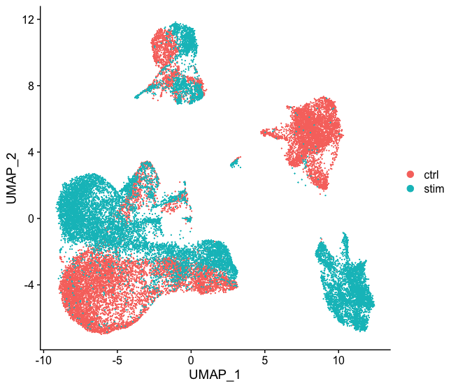
How do we create this UMAP?
The UMAP above can be generated by using the `seurat_phase` object from the previous lesson. For this object we have already run PCA, so the next steps would be to `RunUMAP()` and then plot, as shown in the code below.
# Run UMAP
seurat_phase <- RunUMAP(seurat_phase,
                        dims = 1:40,reduction = "pca")
# Plot UMAP
DimPlot(seurat_phase)
Condition-specific clustering of the cells indicates that we need to integrate the cells across conditions to ensure that cells of the same cell type cluster together.
Why is it important the cells of the same cell type cluster together?
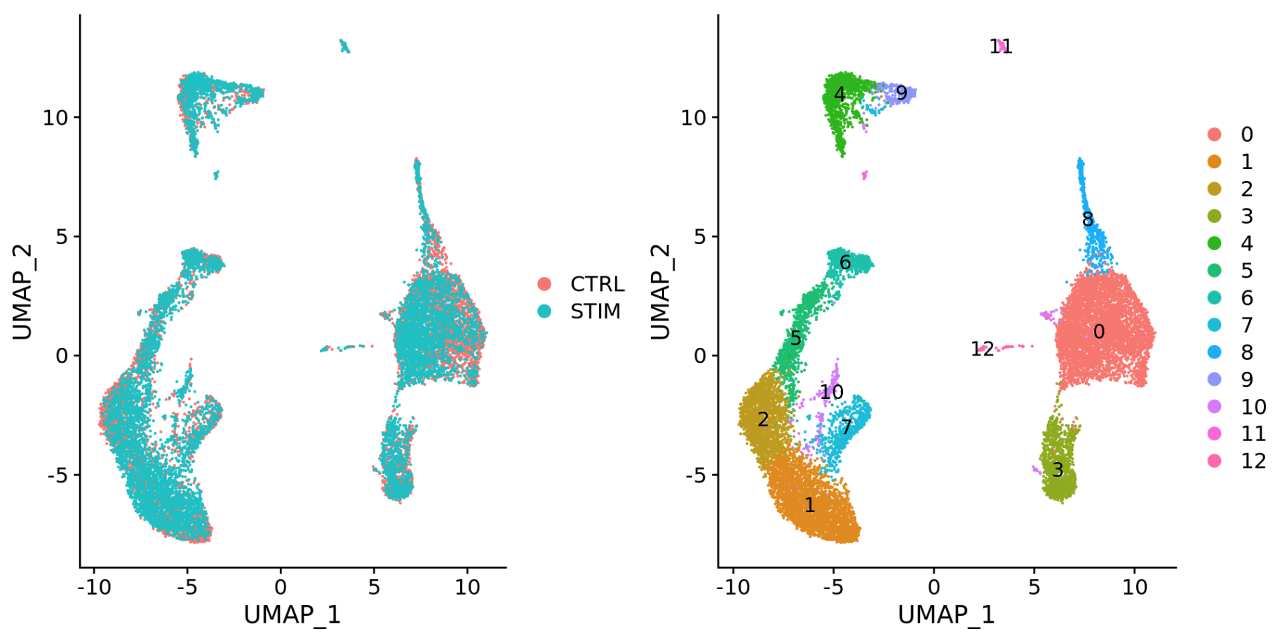
We want to identify cell types which are present in all samples/conditions/modalities within our dataset, and therefore would like to observe a representation of cells from both samples/conditions/modalities in every cluster. This will enable more interpretable results downstream (i.e. DE analysis, ligand-receptor analysis, differential abundance analysis…).
In this lesson, we will cover the integration of our samples across conditions, which is adapted from the Seurat Guided Integration Tutorial.
NOTE: Seurat has a vignette for how to run through the workflow from normalization to clustering without integration. Other steps in the workflow remain fairly similar, but the samples would not necessarily be split in the beginning and integration would not be performed.
It can help to first run conditions individually if unsure what clusters to expect or expecting some different cell types between conditions (e.g. tumor and control samples), then run them together to see whether there are condition-specific clusters for cell types present in both conditions. Oftentimes, when clustering cells from multiple conditions there are condition-specific clusters and integration can help ensure the same cell types cluster together.
Integrate or align samples across conditions using shared highly variable genes
If cells cluster by sample, condition, batch, dataset, modality, this integration step can greatly improve the clustering and the downstream analyses.
To integrate, we will use the shared highly variable genes (identified using SCTransform) from each group, then, we will “integrate” or “harmonize” the groups to overlay cells that are similar or have a “common set of biological features” between groups. For example, we could integrate across:
-
Different conditions (e.g. control and stimulated)
-
Different datasets (e.g. scRNA-seq from datasets generated using different library preparation methods on the same samples)
-
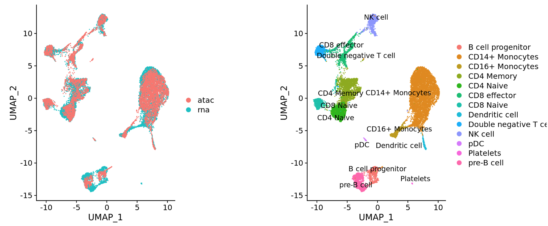
Different modalities (e.g. scRNA-seq and scATAC-seq)
-
Different batches (e.g. when experimental conditions make batch processing of samples necessary)
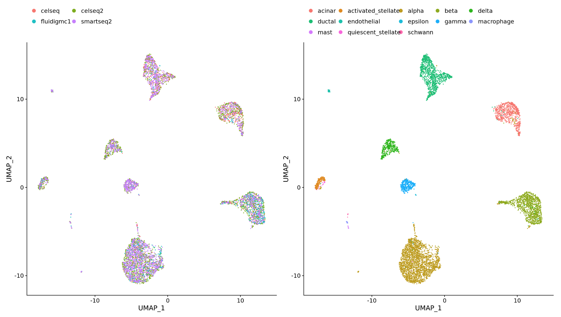
Integration is a powerful method that uses these shared sources of greatest variation to identify shared subpopulations across conditions or datasets [Stuart and Bulter et al. (2018)]. The goal of integration is to ensure that the cell types of one condition/dataset align with the same celltypes of the other conditions/datasets (e.g. control macrophages align with stimulated macrophages).
Integration using CCA
The integration method that is available in the Seurat package utilizes the canonical correlation analysis (CCA). This method expects “correspondences” or shared biological states among at least a subset of single cells across the groups. The steps in the Seurat integration workflow are outlined in the figure below:
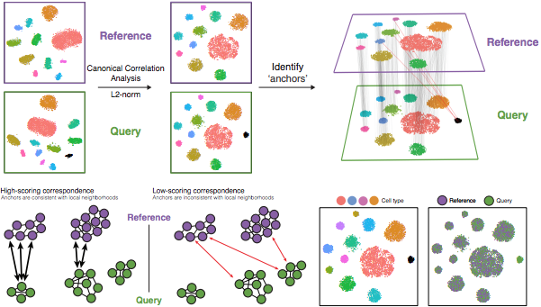
Image credit: Stuart T and Butler A, et al. Comprehensive integration of single cell data, bioRxiv 2018 (https://doi.org/10.1101/460147)
The different steps applied are as follows:
-
Perform canonical correlation analysis (CCA):
CCA identifies shared sources of variation between the conditions/groups. It is a form of PCA, in that it identifies the greatest sources of variation in the data, but only if it is shared or conserved across the conditions/groups (using the 3000 most variant genes from each sample).
This step roughly aligns the cells using the greatest shared sources of variation.
NOTE: The shared highly variable genes are used because they are the most likely to represent those genes distinguishing the different cell types present.
-
Identify anchors or mutual nearest neighbors (MNNs) across datasets (sometimes incorrect anchors are identified):
MNNs can be thought of as ‘best buddies’. For each cell in one condition:
- The cell’s closest neighbor in the other condition is identified based on gene expression values - its ‘best buddy’.
- The reciprocal analysis is performed, and if the two cells are ‘best buddies’ in both directions, then those cells will be marked as anchors to ‘anchor’ the two datasets together.
“The difference in expression values between cells in an MNN pair provides an estimate of the batch effect, which is made more precise by averaging across many such pairs. A correction vector is obtained and applied to the expression values to perform batch correction.” [Stuart and Bulter et al. (2018)].
-
Filter anchors to remove incorrect anchors:
Assess the similarity between anchor pairs by the overlap in their local neighborhoods (incorrect anchors will have low scores) - do the adjacent cells have ‘best buddies’ that are adjacent to each other?
-
Integrate the conditions/datasets:
Use anchors and corresponding scores to transform the cell expression values, allowing for the integration of the conditions/datasets (different samples, conditions, datasets, modalities)
NOTE: Transformation of each cell uses a weighted average of the two cells of each anchor across anchors of the datasets. Weights determined by cell similarity score (distance between cell and k nearest anchors) and anchor scores, so cells in the same neighborhood should have similar correction values.
If cell types are present in one dataset, but not the other, then the cells will still appear as a separate sample-specific cluster.
This lesson has been developed by members of the teaching team at the Harvard Chan Bioinformatics Core (HBC). These are open access materials distributed under the terms of the Creative Commons Attribution license (CC BY 4.0), which permits unrestricted use, distribution, and reproduction in any medium, provided the original author and source are credited.
- A portion of these materials and hands-on activities were adapted from the Satija Lab’s Seurat - Guided Clustering Tutorial