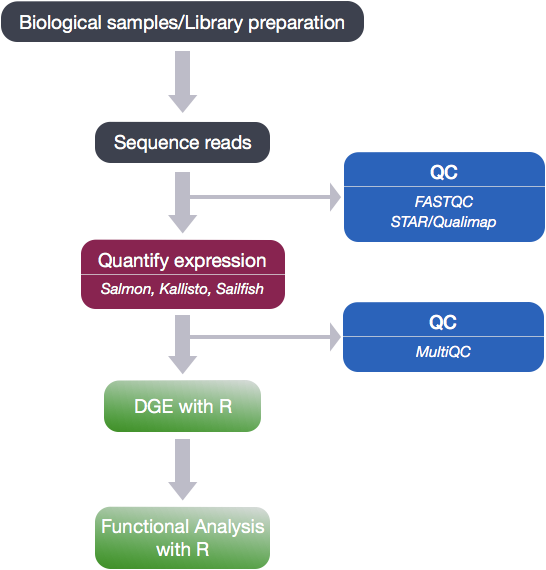
Analysis workflow
The goal of RNA-seq is often to perform differential expression testing to determine which genes or transcripts are expressed at different levels between conditions. These findings can offer biological insight into the processes affected by the condition(s) of interest. Below is an overview of the analysis workflow that is followed for differential gene expression analysis with bulk RNA-seq data.
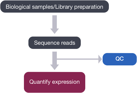
QC on sequencing data
The first step in the RNA-Seq workflow is to take the FASTQ files received from the sequencing facility and assess the quality of the reads.
Unmapped read data (FASTQ)
The FASTQ file format is the defacto file format for sequence reads generated from next-generation sequencing technologies. This file format evolved from FASTA in that it contains sequence data, but also contains quality information. Similar to FASTA, the FASTQ file begins with a header line. The difference is that the FASTQ header is denoted by a @ character. For a single record (sequence read) there are four lines, each of which are described below:
| Line | Description |
|---|---|
| 1 | Always begins with ‘@’ and then information about the read |
| 2 | The actual DNA sequence |
| 3 | Always begins with a ‘+’ and sometimes the same info in line 1 |
| 4 | Has a string of characters which represent the quality scores; must have same number of characters as line 2 |
Let’s use the following read as an example:
@HWI-ST330:304:H045HADXX:1:1101:1111:61397
CACTTGTAAGGGCAGGCCCCCTTCACCCTCCCGCTCCTGGGGGANNNNNNNNNNANNNCGAGGCCCTGGGGTAGAGGGNNNNNNNNNNNNNNGATCTTGG
+
@?@DDDDDDHHH?GH:?FCBGGB@C?DBEGIIIIAEF;FCGGI#########################################################
As mentioned previously, line 4 has characters encoding the quality of each nucleotide in the read. The legend below provides the mapping of quality scores (Phred-33) to the quality encoding characters. Different quality encoding scales exist (differing by offset in the ASCII table), but note the most commonly used one is fastqsanger.
 Quality encoding: !"#$%&'()*+,-./0123456789:;<=>?@ABCDEFGHI
                   |         |         |         |         |
    Quality score: 0........10........20........30........40
Each quality score represents the probability that the corresponding nucleotide call is incorrect. This quality score is logarithmically based and is calculated as:
Q = -10 x log10(P), where P is the probability that a base call is erroneous
These probability values are assigned by the base calling algorithm. The score values can be interpreted as follows:
| Phred Quality Score | Probability of incorrect base call | Base call accuracy |
|---|---|---|
| 10 | 1 in 10 | 90% |
| 20 | 1 in 100 | 99% |
| 30 | 1 in 1000 | 99.9% |
| 40 | 1 in 10,000 | 99.99% |
Therefore, for the first nucleotide in the read (C), there is less than a 1 in 1000 chance that the base was called incorrectly. Whereas, for the the end of the read there is greater than 50% probability that the base is called incorrectly.
Assessing quality with FastQC
Now that we understand what information is stored in a FASTQ file, let’s talk about using that information to assess quality.
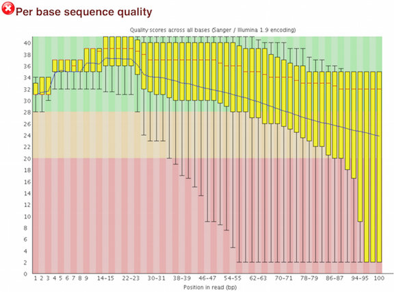
This assessment of read quality is not performed manually; there are tools to help examine the quality metrics. FastQC is one of the most common tools for this step of the workflow. It provides a modular set of analyses, with clear visualizations, to provide a quick impression of whether the data has any problems of which one should be aware of before proceeding with any further analysis.
A few examples of assessments performed by FastQC are:
- aggregate read quality information and plot box plots
- levels of overrepresentation
- GC%
FastQC has a really well documented manual page with more details about all the plots in the report. We recommend looking at this post for more information on what bad plots look like and what they mean for your data.
We also have a slidedeck of error profiles for Illumina sequencing, where we discuss specific FASTQC plots and possible sources of these types of errors.
The “Per base sequence quality” plot is the most commonly used one and it provides the distribution of quality scores across all bases at each position in the reads.
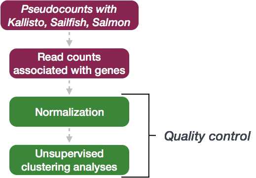
Expression quantification
Once it has been determined that the read quality is good, the next step is to quantify gene expression.
Tools that have been found to be most accurate for this step in the analysis are referred to as lightweight alignment tools, which include Kallisto, Sailfish and Salmon; each working slightly different from one another. Salmon and Kallisto are equally good choices with similar performance metrics for speed and accuracy.
Common to all of these tools is that base-to-base alignment of the reads to the reference genome is avoided, which is the time- and memory-consuming function of splice-aware alignment tools such as STAR and HISAT2. The lightweight alignment tools provide quantification estimates much faster (typically more than 20 times faster) with improvements in accuracy [1]. These transcript expression estimates, often referred to as ‘pseudocounts’ or ‘abundance estimates’, can be aggregated to the gene level for use with differential gene expression tools like DESeq2 or the estimates can be used directly for splice-isoform differential expression using a tool like Sleuth.
Expression data :: Normalization and QC
Once expression is quantified and counts are generated, the next step is more QC! The next few steps in the analysis are shown in the flowchart below.
Normalization of count data
The first step in the DE analysis workflow is count normalization, which is necessary to make accurate comparisons of gene expression between samples.
The counts of mapped reads for each gene is proportional to the expression of RNA (“interesting”) in addition to many other factors (“uninteresting”). Normalization is the process of scaling raw count values to account for the “uninteresting” factors. In this way the expression levels are more comparable between and within samples.
The main factors often considered during normalization are:
-
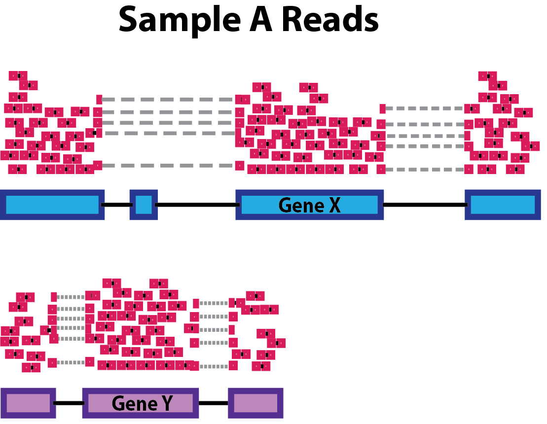
Sequencing depth: Accounting for sequencing depth is necessary for comparison of gene expression between samples. In the example below, each gene appears to have doubled in expression in Sample A relative to Sample B, however this is a consequence of Sample A having double the sequencing depth.
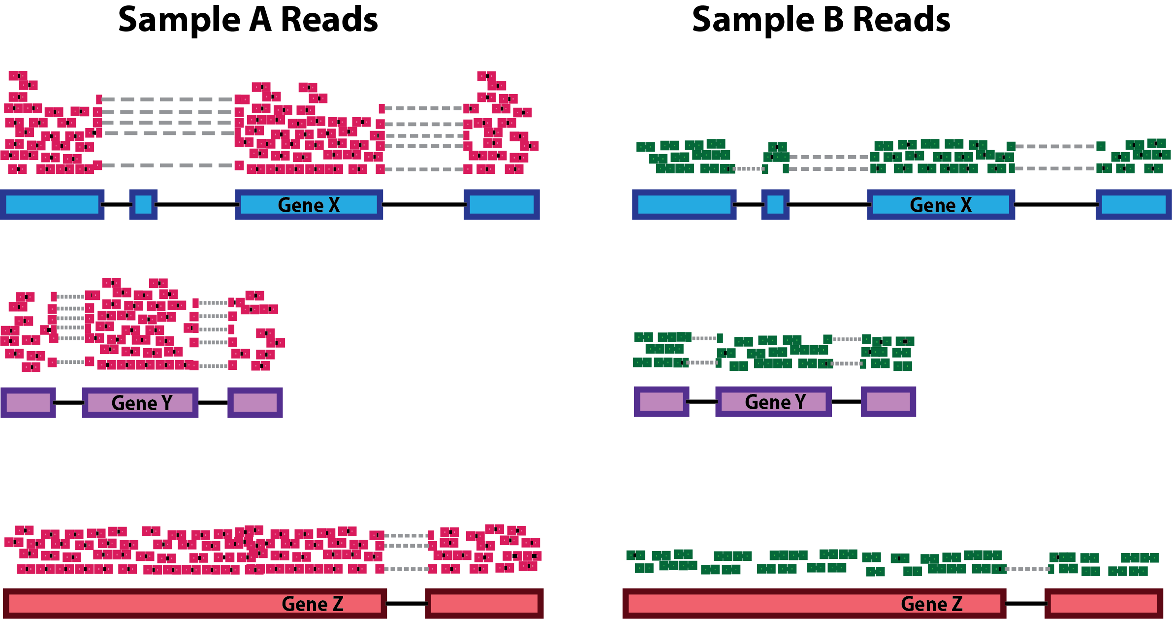
NOTE: In the figure above, each pink and green rectangle represents a read aligned to a gene. Reads connected by dashed lines connect a read spanning an intron.
-
Gene length: Accounting for gene length is necessary for comparing expression between different genes within the same sample. In the example, Gene X and Gene Y have similar levels of expression, but the number of reads mapped to Gene X would be many more than the number mapped to Gene Y because Gene X is longer.
-
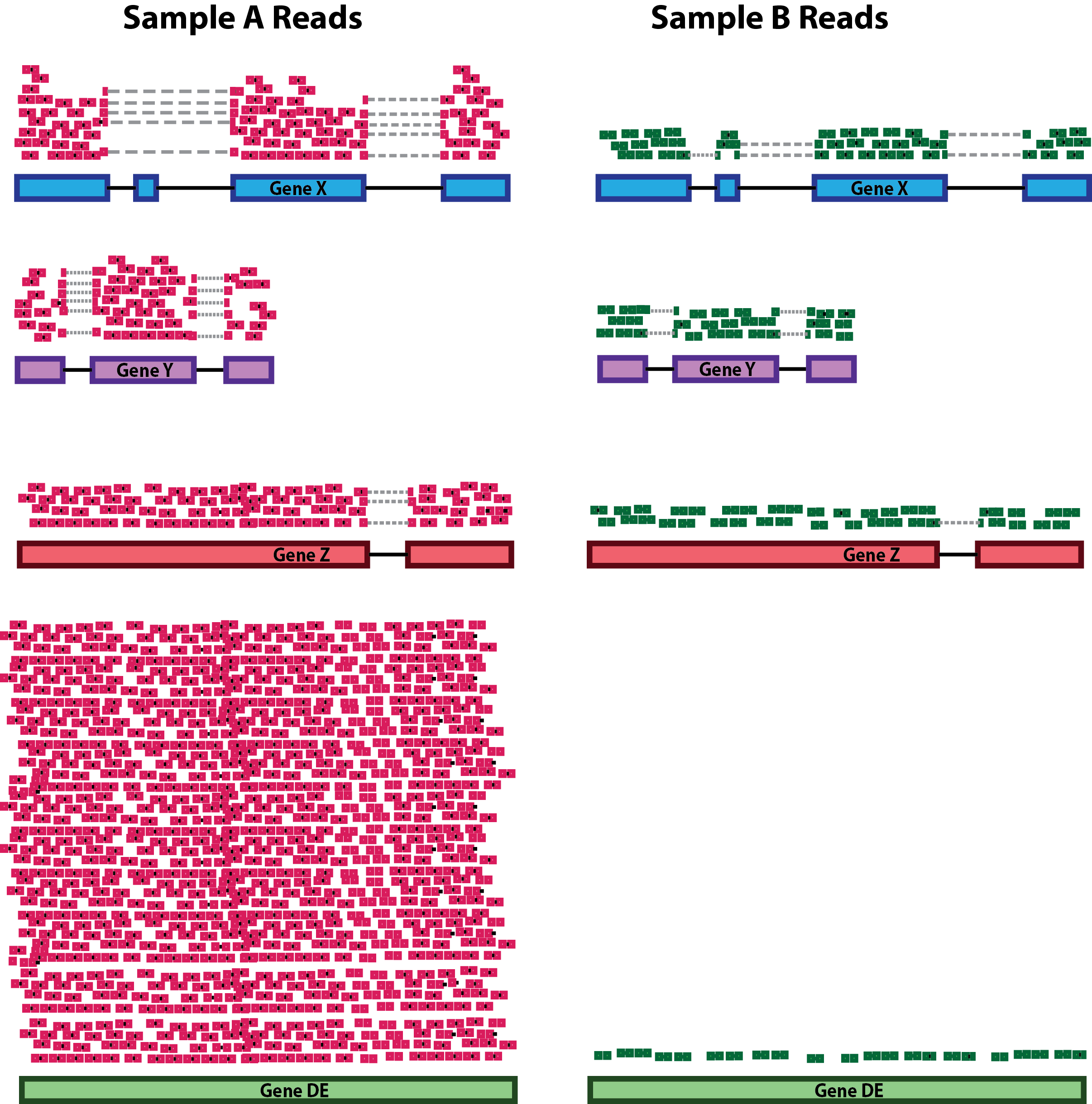
RNA composition: A few highly differentially expressed genes between samples, differences in the number of genes expressed between samples, or presence of contamination can skew some types of normalization methods. Accounting for RNA composition is recommended for accurate comparison of expression between samples, and is particularly important when performing differential expression analyses [1].
In the example, if we were to divide each sample by the total number of counts to normalize, the counts would be greatly skewed by the DE gene, which takes up most of the counts for Sample A, but not Sample B. Most other genes for Sample A would be divided by the larger number of total counts and appear to be less expressed than those same genes in Sample B.
While normalization is essential for differential expression analyses, it is also necessary for QC, exploratory data analysis, visualization of data, and whenever you are exploring or comparing counts between or within samples.
Common normalization methods
Several common normalization methods exist to account for these differences:
Normalization method Description Accounted factors Recommendations for use CPM (counts per million) counts scaled by total number of reads sequencing depth gene count comparisons between replicates of the same samplegroup; NOT for within sample comparisons or DE analysis TPM (transcripts per kilobase million) counts per length of transcript (kb) per million reads mapped sequencing depth and gene length gene count comparisons within a sample or between samples of the same sample group; NOT for DE analysis RPKM/FPKM (reads/fragments per kilobase of exon per million reads/fragments mapped) similar to TPM sequencing depth and gene length gene count comparisons between genes within a sample; NOT for between sample comparisons or DE analysis DESeq2’s median of ratios [1] counts divided by sample-specific size factors determined by median ratio of gene counts relative to geometric mean per gene sequencing depth and RNA composition gene count comparisons between samples and for DE analysis; NOT for within sample comparisons EdgeR’s trimmed mean of M values (TMM) [2] uses a weighted trimmed mean of the log expression ratios between samples sequencing depth, RNA composition gene count comparisons between samples and for DE analysis; NOT for within sample comparisons NOTE: This video by StatQuest shows in more detail why TPM should be used in place of RPKM/FPKM if needing to normalize for sequencing depth and gene length.
Quality Control
The next step in the differential expression workflow is QC, which includes sample-level and gene-level steps to perform QC checks on the count data to help us ensure that the samples/replicates look good and to help identify problematic expression trends and outliers. Normalized counts are utilized for this step.
Sample-level QC
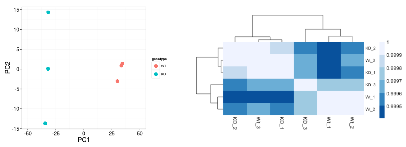
A useful initial step in an RNA-seq analysis is often to assess overall similarity between samples:
- Which samples are similar to each other, which are different?
- Does this fit to the expectation from the experiment’s design?
- What are the major sources of variation in the dataset?
Sample-level QC allows us to see how well our replicates cluster together, as well as, observe whether our experimental condition represents the major source of variation in the data. Performing sample-level QC can also identify any sample outliers, which may need to be explored to determine whether they need to be removed prior to DE analysis.
The 2 main methods utilized for this type of QC are Principal Component Analysis (PCA) and Hierarchical Clustering (and correlation between samples).
Gene-level QC
In addition to examining how well the samples/replicates cluster together, there are a few more QC steps. Prior to differential expression analysis it is beneficial to omit genes that have little or no chance of being detected as differentially expressed. This will increase the power to detect differentially expressed genes. The genes omitted fall into three categories:
- Genes with zero counts in all samples
- Genes with an extreme count outlier
- Genes with a low mean normalized counts
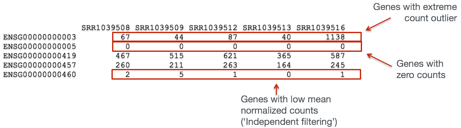
Some statistical tools, e.g. DESeq2, used for identifying differentially expressed genes will perform this filtering by default; however other tools, e.g. EdgeR, will not.
Count modeling and statistical analysis
The final step in the differential expression analysis workflow is fitting the counts to a model and performing the statistical test for differentially expressed genes. In this step we essentially want to determine whether the mean expression levels of different sample groups are significantly different.
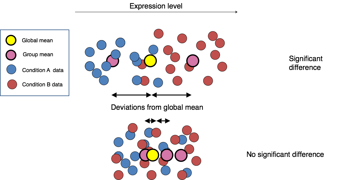
Image credit: Paul Pavlidis, UBC
Some highlights of RNA-seq count data
- a large proportion of the genes have low values associated with them
- there is no upper limit for expression (large dynamic range)
- the negative binomial model has been determined to be the best fit for the count distribution for RNA-seq data where there is a lot of variance between the replicates and mean < variance
Tools for statistical analysis
There are a number of software packages that have been developed for differential expression analysis of RNA-seq data. A few tools are generally recommended as best practice, e.g. DESeq2 and EdgeR. Both these R packages use the negative binomial model, employ similar methods, and typically, yield similar results. They are pretty stringent, and have a good balance between sensitivity and specificity (reducing both false positives and false negatives).
Limma-Voom is another set of tools often used together for DE analysis, but this method may be less sensitive for small sample sizes. This method is recommended when the number of biological replicates per group grows large (> 20).
Further reading about DGE tool comparisons.
Note, these tools make the assumption that majority of the genes are not different between the sample groups.
Multiple test correction
The output of any of these analysis methods is a p-value as well as a value assigning statistical significance after multiple test correction, and the second value is what should be used when creating lists of genes that are differentially expressed.
Each p-value returned is the result of a single test (single gene). If we used the p-value directly with a significance cut-off of p < 0.05, that means there is a 5% chance it is a false positive and the more genes we test, the more we inflate the false positive rate. For example, if we test 20,000 genes for differential expression, at p < 0.05 we would expect to find 1,000 genes by chance. If we found 3000 genes to be differentially expressed total, roughly one third of our genes are false positives. We would not want to sift through our “significant” genes to identify which ones are true positives.
A few common methods to correct for multiple testing are listed below:
- Bonferroni: The adjusted p-value is calculated by: p-value * m (m = total number of tests). This is a very conservative approach with a high probability of false negatives, so is generally not recommended.
- FDR/Benjamini-Hochberg: Benjamini and Hochberg (1995) defined the concept of FDR and created an algorithm to control the expected FDR below a specified level given a list of independent p-values. An interpretation of the BH method for controlling the FDR is implemented in DESeq2 in which we rank the genes by p-value, then multiply each ranked p-value by m/rank.
- Q-value / Storey method: The minimum FDR that can be attained when calling that feature significant. For example, if gene X has a q-value of 0.013 it means that 1.3% of genes that show p-values at least as small as gene X are false positives