NOTE: This lesson was adapted from Dr. Mary Piper’s presentation for the Boston-area Women’s Bioinformatics Meetup.
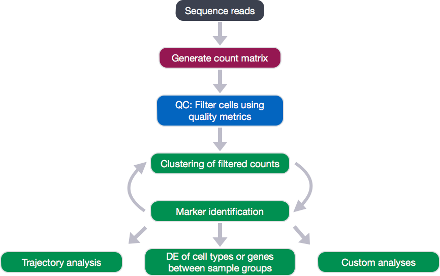
Single-cell RNA-seq analysis workflow
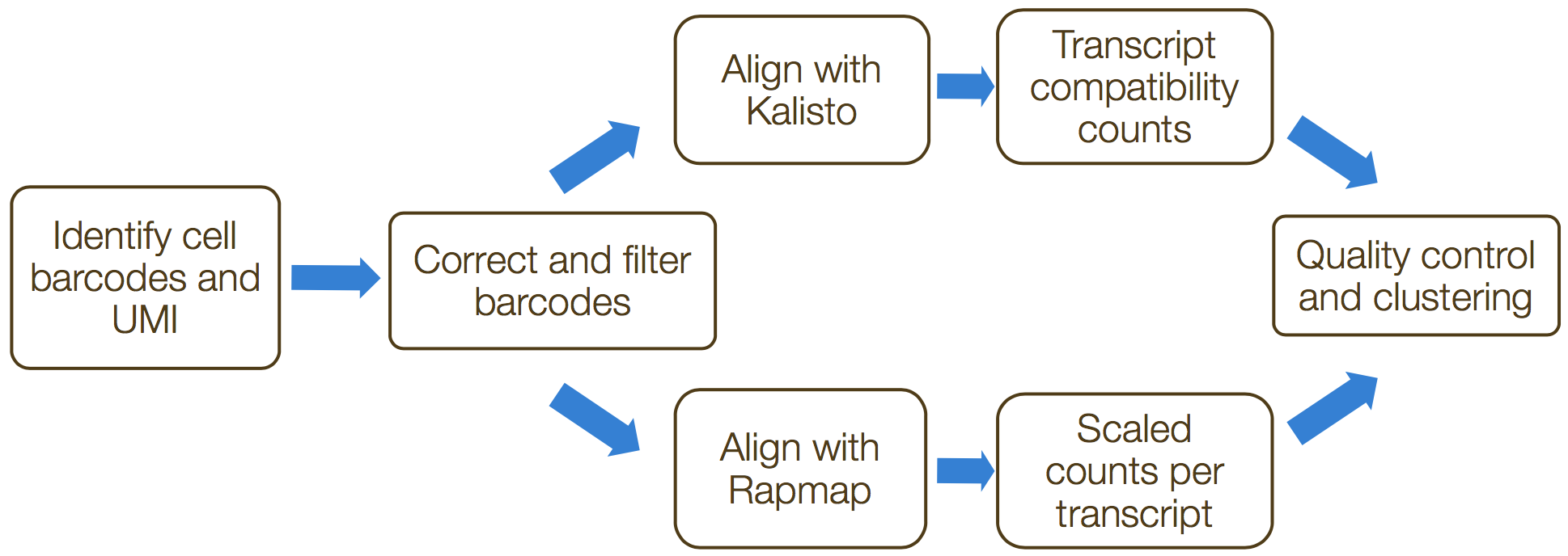
Count matrix generation
The scRNA-seq method will determine how to generate the count matrix using technology-specific methods to parse the barcodes and UMIs from the sequencing reads so as to delineate the cells and the transcripts.
’umis provides tools for estimating expression in RNA-seq data which performs sequencing of end tags of transcript, and incorporate molecular tags to correct for amplification bias.’ The steps in this process include the following:
- Formatting reads and filtering noisy cellular barcodes
- Demultiplexing the samples
- Pseudo-mapping to cDNAs
- Counting molecular identifiers

The generation of the count matrix from the raw sequencing data follow the steps in the schematic below for many of the scRNA-seq methods.
Following the generation of count matrix, the remaining steps can be performed using Seurat, the R toolkit for single cell genomics. A tutorial for the remaining steps can be found here, and requires a good working knowledge of R.
Filtering
Poor quality cells can be filtered out of the count matrix data before moving forward. Poor quality cells often have the following characteristics:
- a low number of genes or UMIs
- high mitochondrial gene expression indicative of dying cells
- low number of genes per UMI.
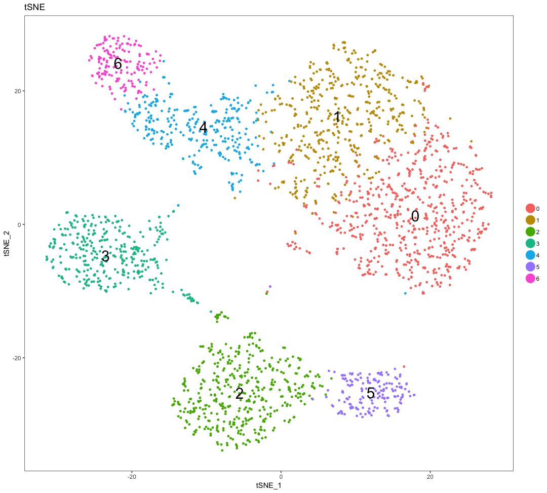
Clustering
After removing the poor quality cells, the cells can now be clustered based on similarities in transcriptional activity, with the idea that the different cell types separate into the different clusters. The following steps can be followed to perform clustering:
- Normalization and transformation of the raw gene counts per cell to account for differences in sequencing depth per cell.
- Identification of high variance genes.
- Regression of sources of unwanted variation (e.g. number of UMIs per cell, mitochondrial transcript abundance, cell cycle phase).
- Identification of the primary sources of heterogeneity using principal component (PC) analysis and heatmaps.
- Clustering cells based on significant PCs.
To visualize the clusters, there are a few different options that can be helpful, including t-distributed stochastic neighbor embedding (t-SNE), Uniform Manifold Approximation and Projection (UMAP), and PCA. The goals of these methods is to have similar cells closer together in low-dimensional space.
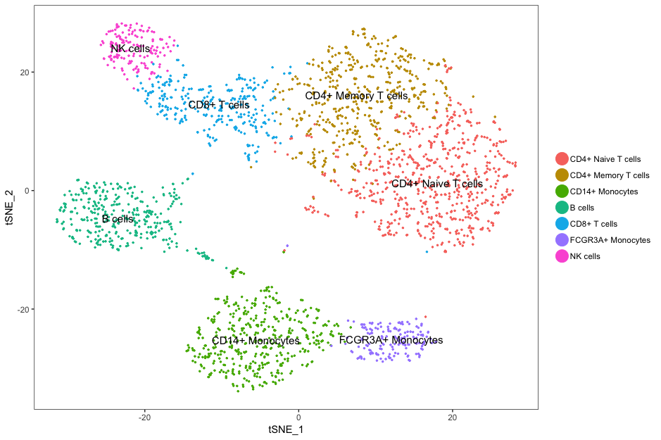
Marker identification
After clustering, genes that are markers for different clusters can be used to help identify the cell type of each cluster. Finally, after identification of cell types, there are various types of analyses that can be performed depending on the goal of the experiment.
This lesson was adapted from Dr. Mary Piper’s presentation for the Boston-area Women’s Bioinformatics Meetup.
This lesson has been developed by members of the teaching team at the Harvard Chan Bioinformatics Core (HBC). These are open access materials distributed under the terms of the Creative Commons Attribution license (CC BY 4.0), which permits unrestricted use, distribution, and reproduction in any medium, provided the original author and source are credited.