Learning Objectives

• Use code chunk options to customize the report
• Describe how to add figures and tables to an RMarkdown
• Describe how to specify the output format for RMarkdown

More about Code chunks

By this point, we have mentioned the word “knit” quite a few times, and you have installed and loaded the knitr package too. But, we have not yet fully defined what it is. knitr is an R package, developed by Yihui Xie, designed to convert RMarkdown and a couple of other file formats into a final report document in HTML or PDF or other formats.

The knitr package provides a lot of customization options for code chunks embedded within the file. These options are written in the form of tag=value.

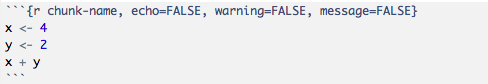
There is a comprehensive list of all the available options, however when starting out this can be overwhelming. Here, we provide a short list of some options commonly used in code chunks:

• echo = TRUE: whether to include R source code in the final knitted document. If echo = FALSE, R source code will not be written. But the code is still evaluated and its output will be included in the final document.
• eval = TRUE: whether to evaluate/execute the code.
• include = TRUE: whether to include R source code and its output in the final document. If include = FALSE, nothing (R source code and its output) will be written into the final document. But the code is still evaluated and plot files are generated if there are any plots in the chunk.
• warning = TRUE: whether to preserve warnings in the output like we run R code in a terminal (if FALSE, all warnings will be printed in the console instead of the output document).
• message = TRUE: whether to preserve messages emitted by message() in the final output document (similar to warning).
• results = "asis": output as-is, i.e., write raw results from R into the output document instead of LaTeX-formatted output. Another useful option for this option is “hide”, which will hide the results, or all normal R output.

Global options

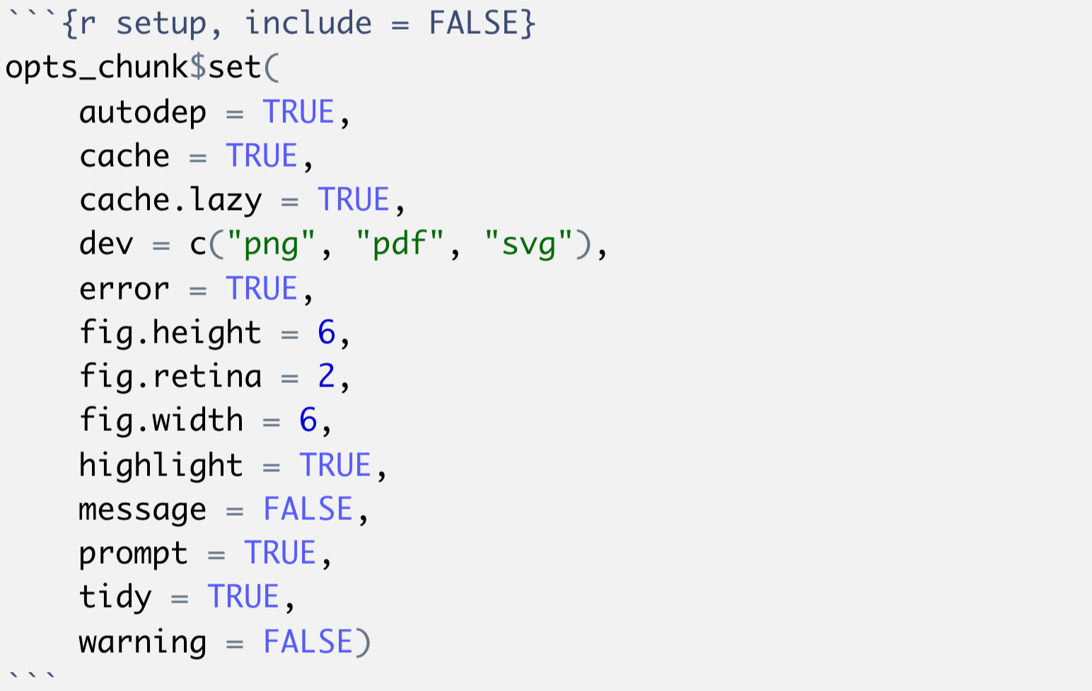
knitr also allows for global options, which means choosing options that apply to all code chunks in an RMarkdown file. These will be the default options used for all the code chunks in the document, unless a modification is specified in an individual code chunk.

Global options should be placed inside your setup code chunk. The setup chunk is a special knitr chunk that should be placed at the start of the document. We recommend storing all library() loads required for the script in this setup chunk too!

NOTE: An additional cool trick is that you can save opts_chunk$set settings in a hidden file called .Rprofile. This file is located in your home directory and accessed by RStudio everytime your open up a new session. By setting this up, these knitr options will apply to all of your RMarkdown documents that you create.

---

Exercise #3

1. Only some of the code chunks in the workshop-example.Rmd file have names; go through and add names to the unnamed code chunks.
2. For the code chunk named data-ordering do the following:
   • First, add a new line of code to display first few rows of the newly created data_ordered data frame. You may use head() function here.
   • Next, modify the options for ({r data-ordering}) such that in the knitted report, the output from the new line of code will show up, but the code is hidden.
3. Without removing the second-to-last code chunk ({r boxplot}) from the Rmd file, modify its options such that neither the code nor its output appear in the report
4. knit the markdown

Answer Key

---

Adding figures

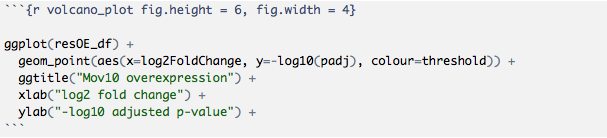
A neat feature of knitr is how much simpler it is to generate and add figures to a report! For the most part, you don’t need to do anything special, just add a code chunk that generates a figure. When the file is knit, the figure will automatically be produced and inserted into the final document. A single chunk can support multiple plots, and they will be appear one after the other below the chunk.

There are a few code chunk options commonly used for plots. For example, to easily resize the figures in the final report, you can specify the fig.height and fig.width of the figure when setting up the code chunk.

In addition to displaying it in the report, you can also have knitr automatically write the files to a subfolder by using the code chunk option dev.

Adding tables

knitr includes a simple but powerful function for generating stylish tables in a knit report named kable(). Here’s an example using R’s built-in mtcars dataset:

help("kable", "knitr")
mtcars %>%
    head %>%
    kable

	mpg	cyl	disp	hp	drat	wt	qsec	vs	am	gear	carb
Mazda RX4	21.0	6	160	110	3.90	2.620	16.46	0	1	4	4
Mazda RX4 Wag	21.0	6	160	110	3.90	2.875	17.02	0	1	4	4
Datsun 710	22.8	4	108	93	3.85	2.320	18.61	1	1	4	1
Hornet 4 Drive	21.4	6	258	110	3.08	3.215	19.44	1	0	3	1
Hornet Sportabout	18.7	8	360	175	3.15	3.440	17.02	0	0	3	2
Valiant	18.1	6	225	105	2.76	3.460	20.22	1	0	3	1

There are some other functions that allow for more powerful customization of tables, including pander::pander() and xtable::xtable(), but the simplicity and cross-platform reliability of knitr::kable() makes it an easy pick.

Working directory behavior

knitr redefines the working directory of an RMarkdown file in a manner that can be confusing. Make sure that any paths to files specified in the RMarkdown document is relative to its location, and not relative to your current working directory.

A simple way to make sure that the paths are not an issue is by creating an R project for the analysis, and saving all RMarkdown files at the top level and referring to the data and output files within the project directory. This will prevent unexpected problems related to this behavior.

---

This lesson has been developed by members of the teaching team and Michael J. Steinbaugh at the Harvard Chan Bioinformatics Core (HBC). These are open access materials distributed under the terms of the Creative Commons Attribution license (CC BY 4.0), which permits unrestricted use, distribution, and reproduction in any medium, provided the original author and source are credited.