Learning Objective
- Implement external packages to create Venn diagrams and heatmaps
External packages for figure creation
We have discovered that ggplot2 has incredible functionality and versatility; however, there are some examples of visualization that are either not possible at all or require some assistance from external packages. There are a plethora of different packages that specialize in particular types of figures. The Data to Viz resource provides popular packages for specialized plots along with the code to create them.
Visualizing overlaps of sets using Venn diagrams
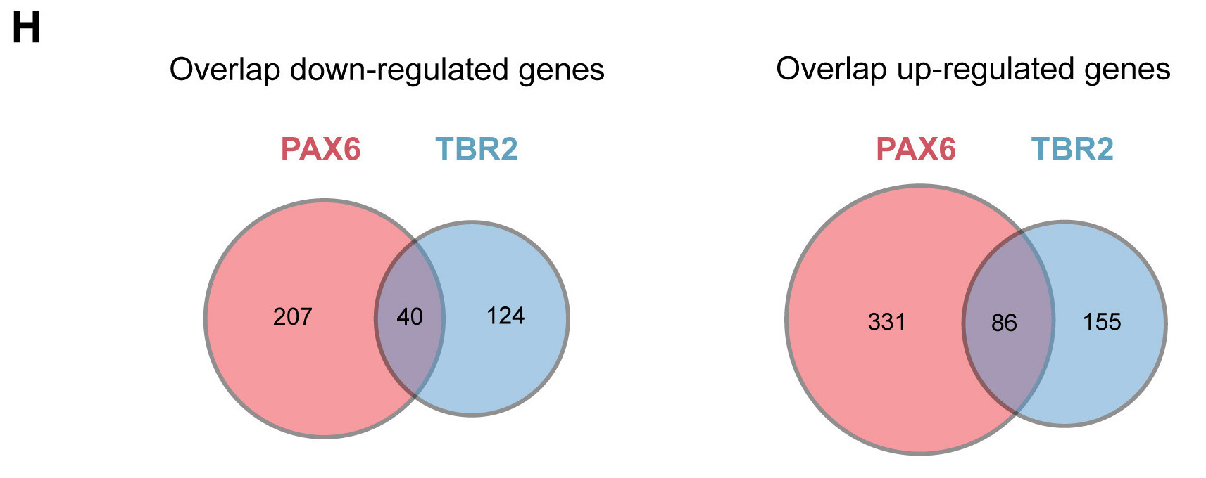
Let’s start by exploring how to create the Venn diagram in figure 4H.
A Venn diagram compares two or more lists, and by nature is categoric. If we use the Data to Viz resource, we can navigate to the Categoric data, and under ‘Two independent lists’ we find the Venn diagram. Clicking on the Venn diagram icon will open up a pop up window with a brief description of Venn diagrams. At the bottom of the pop up page, find the link to the “dedicated page”; explore the dedicated page.
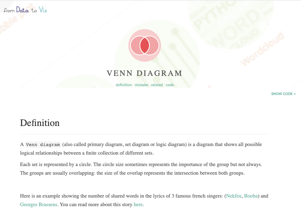
This page has a lot of nice information about Venn diagrams, as well as, suggestions for when to use them (e.g. generally not recommended for comparison of more than 3 sets - use upset plots instead). Since we are comparing two sets of data for each visualization (e.g. Pax6 and Tbr2-expressing samples), a Venn diagram is a recommended method.
If we expand the ‘Code’, we see that the package used to create the Venn diagrams is VennDiagram. Since this is the package used to create the figure in the paper, we will provide code to demonstrate how it was done later in the lesson.
We will focus on the ggvenn package, which provides an easy-to-use way to draw Venn diagrams using the standard ggplot2 syntax and layout. The package hence makes it possible to match the design and style of Venn diagrams to other graphics created by the ggplot2 package.
First, we will need to load the library:
# Load library
library(ggvenn)
To create the Venn diagram, we need to generate our sets. We can subset our data for the Pax6- and Tbr2-expressing samples to only include those genes that are significant with threshold equal to TRUE and that are up-regulated using the log2FoldChange values > 0.
# Up-regulated gene sets for Pax6 and Tbr2
up_pax6 <- results[which(results$pax6_threshold & results$pax6_log2FoldChange > 0),]
up_tbr2 <- results[which(results$tbr2_threshold & results$tbr2_log2FoldChange > 0),]
We can do a similar subset for the down-regulated genes, but with log2FoldChange < 0.
# Down-regulated gene sets for Pax6 and Tbr2
down_pax6 <- results[which(results$pax6_threshold & results$pax6_log2FoldChange < 0),]
down_tbr2 <- results[which(results$tbr2_threshold & results$tbr2_log2FoldChange < 0),]
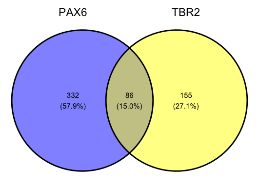
Next, we can use the ggvenn() function from the ggvenn package to create a simple Venn diagram:
# Create list of up-regulated genes
up_list <- list(PAX6 = rownames(up_pax6),
                TBR2 = rownames(up_tbr2))

# Create list of down-regulated genes
down_list <- list(PAX6 = rownames(down_pax6),
                TBR2 = rownames(down_tbr2))
# Create up-regulated Venn diagram
ggvenn(data = up_list)
# Create down-regulated Venn diagram
ggvenn(data = down_list)
Now that we have our venn diagrams of genes that are up- and down-regulated in the respective conditions, we can check how many overlap between the conditions. This is a good check to perform to make sure the packages report the correct interaction numbers.
# Check overlap for upregulated set
length(which(row.names(up_pax6) %in% row.names(up_tbr2)))
# Check overlap for downregulated set
length(which(row.names(down_pax6) %in% row.names(down_tbr2)))
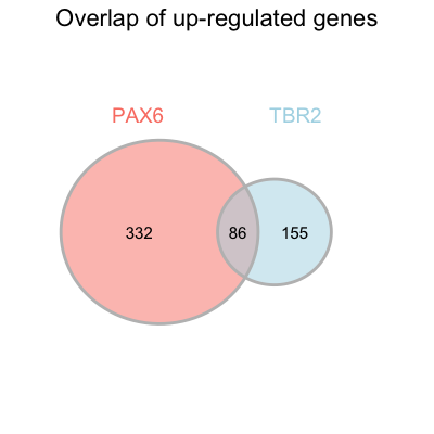
This has successfully created a Venn diagram, but this is not exactly a publication-quality figure. Most obviously, there are changes required to make it more closely resemble the original figure. Let’s explore what we can do with ggvenn.
First, note that since ggvenn is based in ggplot we can add it as a layer just like any other plot. The function geom_venn() comes from the ggvenn package. Note that for most uses, the simple ggvenn() command should suffice but since we have specific changes to replicate the image in the paper, we need to add arguments and/or additional layers. An example of using geom_venn() is provided below:
ggvenn(data = up_list) +
  ggtitle("Overlap of up-regulated genes") +
  theme(plot.title = element_text(hjust = 0.5))
Exercise
Below we provide a skeleton of the publication-quality geom_venn code. The value of the following arguments are left empty:
fill_colorset_name_colorset_name_sizetext_size
Please fill in those values so that the final figure looks similar to that in the paper (see below).
# Up-regulated genes
geom_venn(data = up_list,
          stroke_color="grey",
          show_percentage = FALSE,
          auto_scale = TRUE,
          fill_color= ,
          set_name_color =  ,
          set_name_size = ,
          text_size = ) +
  ggtitle("Overlap of up-regulated genes") +
  theme(plot.title = element_text(hjust = 0.5, size = rel(1.5)))
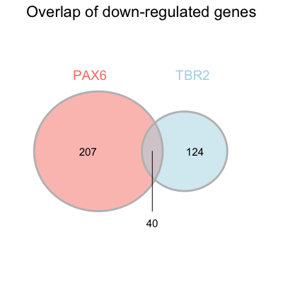
Similarly, we could plot the venn diagram for the down-regulated genes.
Code
    # Create down-regulated venn diagram
    ggvenn(data = down_list,
           stroke_color="grey",
           show_percentage = FALSE,
           auto_scale = TRUE,
           fill_color = c("salmon", "lightblue"),
           set_name_color =  c("salmon", "lightblue"),
           set_name_size = 5,
           text_size = 4,
           stroke_size = 0.01) +
      ggtitle("Overlap of down-regulated genes") +
      theme(plot.title = element_text(hjust = 0.5))
Exporting the VennDiagram
We will need to output our visualization as a pdf or png so that we can later incorporate it into the final figure. We can plot our figure and then call ggsave() to save our plot. Below is an example for our down-regulated genes with a png output.
# Create up-regulated venn diagram
ggvenn(data = up_list,
       stroke_color="grey",
       show_percentage = FALSE,
       auto_scale = TRUE,
       fill_color = c("salmon", "lightblue"),
       set_name_color =  c("salmon", "lightblue"),
       set_name_size = 5,
       text_size = 4) +
  ggtitle("Overlap of up-regulated genes") +
  theme(plot.title = element_text(hjust = 0.5))

# Export up-regulated venn diagram
ggsave("results/venn_up.png")

# Create down-regulated venn diagram
ggvenn(data = down_list,
       stroke_color="grey",
       show_percentage = FALSE,
       auto_scale = TRUE,
       fill_color = c("salmon", "lightblue"),
       set_name_color =  c("salmon", "lightblue"),
       set_name_size = 5,
       text_size = 4) +
  ggtitle("Overlap of down-regulated genes") +
  theme(plot.title = element_text(hjust = 0.5))

# Export down-regulated venn diagram
ggsave("results/venn_down.png")
NOTE: For the down-regulated genes, the overlap number is not placed within the overlapping region. Unfortunately, the placement of this number is not easy to change. To create an identical figure using the
VennDiagrampackage you can check out the link below.
Click here for code to create the figure using the VennDiagram package
    # Load library
    library(VennDiagram)

    # Plot figure
    venn.diagram(x = up_list,
                 filename = "results/venn_up.png",
                 output = TRUE,
                 main = "Overlap of up-regulated genes",
                 main.fontfamily = "sans",
                 main.cex = 0.75,
                 height = 600 ,
                 width = 600 ,
                 resolution = 300,
                 compression = "lzw",
                 lwd = 2,
                 col= "gray",
                 fill = c("salmon", "lightblue"),
                 cex = 0.5,
                 fontfamily = "sans",
                 category.names = c("PAX6" , "TBR2"),
                 cat.cex = 0.7,
                 cat.fontface = "bold",
                 cat.default.pos = "outer",
                 cat.pos = 0,
                 cat.dist = c(0.06,0.097),
                 cat.fontfamily = "sans",
                 cat.col = c("salmon", "lightblue"))
Visualizing numeric data from different conditions or groups
Next, we will generate the Fig 4F heatmap as shown below. We will use specialized packages for the creation of hierarchical heatmaps. A benefit of these packages is that they incorporate statistical information, such as dendrograms and clustering of rows and/or columns. Although ggplot2 can easily create a heatmap with geom_tile(), it cannot easily provide the hierarchical clustering as these packages. A few examples of these packages include pheatmap, d3heatmap, and ComplexHeatmap. We will explore the pheatmap package for our hierarchical clustering figure; however, additional information can be found for d3heatmap from Data to viz, and we have additional materials highlighting the code to create the same plot using ComplexHeatmap. ComplexHeatmap definitely embraces its name, and there is a whole book dedicated to creating custom heatmaps using this package.
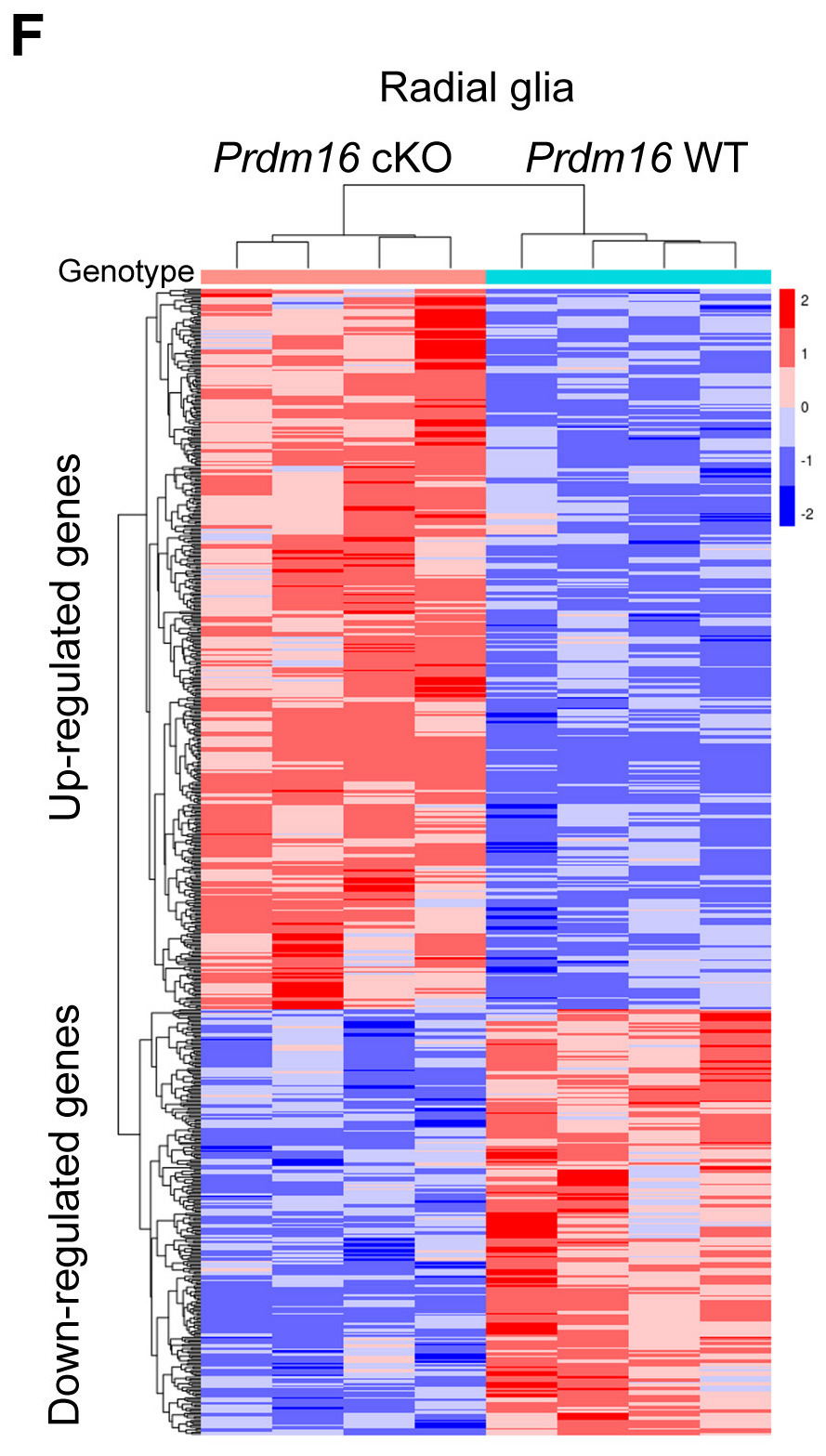
Generally, heatmaps are used to compare numeric data from different conditions or groups. These comparisons range across different fields of study; for instance, a heatmap could be used to explore how temperatures across the seasons have increased over the past 100 years, or it could be used to explore the monthly earnings for all fortune 500 companies. We will use a heatmap to explore our biological data and look at the genes that have significantly different expression between mice with or without the Prdm16 gene. The hierarchical clustering will add information to the figure about which mice are most similar to each other in the expression of these genes.
To create this figure, we first need to subset our gene expression data to the significant genes for the radial glia cells (Pax6-expressers). To get the names of our significant genes we can filter to only include those with significance (p-adjusted) values less than 0.05.
# Get Pax6 sig genes
pax6_sig_genes <- results %>%
  rownames_to_column("ensembl_id") %>%
  filter(pax6_padj < 0.05) %>%
  pull(ensembl_id)
We are only interested in the radial glia, so we will extract only the Pax6 samples.
# Filter heatmap for only the radial glia (Pax6 samples)
heatmap_normCounts <- normalized_counts[ , colnames(normalized_counts)[str_detect(colnames(normalized_counts), "Pax6")]]
Then we can extract only the significant genes from our Pax6 expression matrix.
# Filter for the sig genes
heatmap_normCounts <- heatmap_normCounts[which(rownames(heatmap_normCounts) %in% pax6_sig_genes), ]
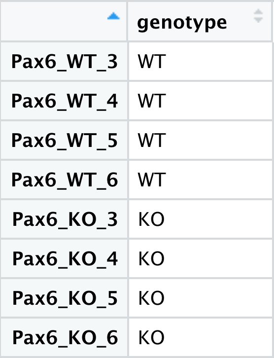
Now we have the values to be included in the heatmap, but we also need to color it by group, Prdm16 knockout or wildtype. To get that information, we need to use our metadata. We will extract the same mice samples from our metadata that we have the counts for, which is the Pax6 samples.
We’ll start by copying our full metadata table to a new variable to ensure we don’t accidently alter our original metadata.
# Copy metadata to new variable
heatmap_meta <- meta
Now to create the heatmap using the pheatmap package, the row names of our metadata need to be the sample names and match the column names of our counts (numeric) data.
# Assign the sample names to be the row names
rownames(heatmap_meta) <- heatmap_meta$samples
Now we can subset the metadata to only include those samples present in the Pax6 counts data.
# Subset metadata to match samples in count data
heatmap_meta <- heatmap_meta[which(rownames(heatmap_meta) %in% colnames(heatmap_normCounts)), ]
We are only interested in using the genotype annotations, so we will keep only that column. All columns given to pheatmap for annotations will be included as separate bars.
# Select only the genotype column for annotations
heatmap_meta <- heatmap_meta %>%
  select(genotype)
The factor levels for the genotype will determine the color automatically assigned to the group. We can manually specify the levels using the factor() function.
# Re-level factors
heatmap_meta$genotype <- factor(heatmap_meta$genotype, levels = c("WT", "KO"))
Now that we have the metadata with information for annotating the groups and the count data to be visually transformed into the heatmap, we only need to provide any customized colors to use in the heatmap and to denote the groups. We can specify the colors to use for the gradient in the numeric expression values:
# Colors for heatmap
heatmap_colors <- colorRampPalette(c("blue", "white", "red"))(6)
Also, we can specify the colors to use to denote the annotations. The colors for the annotations need to be provided as a list:
# Colors for denoting annotations
ann_colors <- list(genotype = c(KO = "#F8766D", WT = "#00BFC4"))
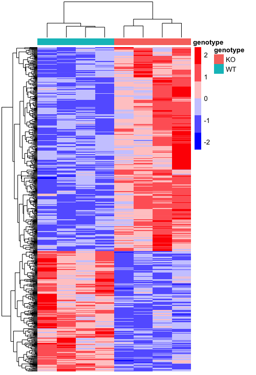
Now we can load the pheatmap library, using the pheatmap() function to create the heatmap.
# Load library
library(pheatmap)

# Plot heatmap
pheatmap(heatmap_normCounts,
         color = heatmap_colors,
         annotation_col = heatmap_meta,
         annotation_colors = ann_colors,
         show_colnames = F,
         show_rownames = F)
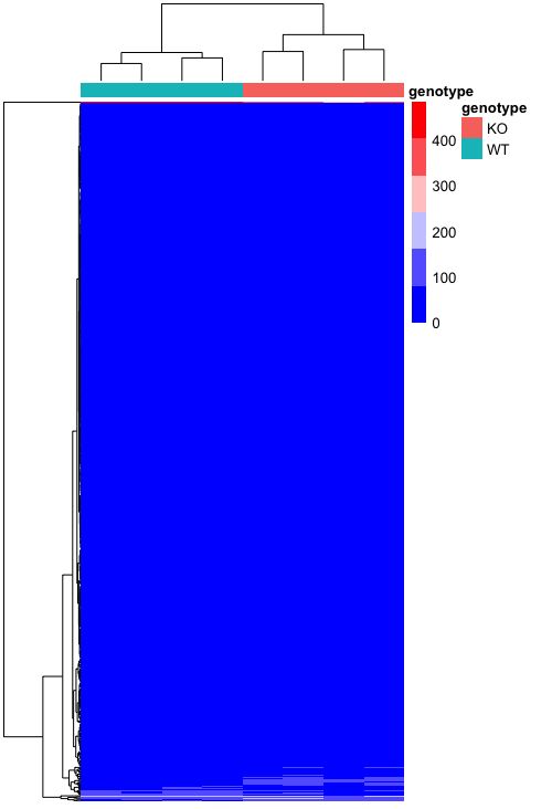
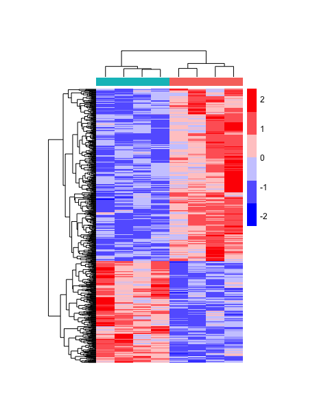
We are have created a basic heatmap, but it’s not very informative as it is. It looks like the expression of a lot of the genes is much lower than some of the others, so we can’t see the differences very easily for the genes that don’t have the highest values. There is a helpful argument called scale that allows us to scale the colors by the values in each row or column. Since each gene is a row, we will add this argument to be scale = "row", which centers and scales the values.
# Plot heatmap scaled by row
pheatmap(heatmap_normCounts,
         color = heatmap_colors,
         annotation_col = heatmap_meta,
         annotation_colors = ann_colors,
         show_colnames = F,
         show_rownames = F,
         scale="row")
Now that looks a lot better! We can see clustering between the different groups, which is good since these genes are supposed to be significantly different in their expression between the groups. We can add a few more arguments to make it look more like the figure, like deleting the annotation name and legend. We will also adjust the width and height of the tiles.
# Scaled heatmap with adjustments for figure
pheatmap(heatmap_normCounts,
         color = heatmap_colors,
         annotation_col = heatmap_meta,
         annotation_colors = ann_colors,
         show_colnames = F,
         show_rownames = F,
         scale="row",
         treeheight_col = 25,
         cellwidth = 20,
         cellheight = 0.4,
         annotation_names_col = F,
         annotation_legend = F)
Now we are only missing the text annotations, and we can add using the cowplot package we learned about earlier. However, the pheatmap image is stored as a list rather than a graphics object. The ggplotify package allows us to manipulate this list object into a ggplot object with the as.ggplot() function, faciliatating further modifications with ggplot2 or cowplot.
# Load library
library(ggplotify)

# Turn into a ggplot object
heatmap <- as.ggplot(pheatmap(heatmap_normCounts,
                              color = heatmap_colors,
                              cluster_rows = T,
                              annotation_col = heatmap_meta,
                              annotation_colors = ann_colors,
                              border_color="white",
                              cluster_cols = T,
                              show_colnames = F,
                              show_rownames = F,
                              scale="row",
                              treeheight_col = 25,
                              cellwidth = 20,
                              cellheight = 0.40,
                              fontsize = 9,
                              annotation_names_col = F,
                              annotation_legend = F))
To add the annotations at the top and left sides of the plot, we will use the theme() function from ggplot2 to add whitespace. With the plot.margin argument we can specify the amount of space to add to the top, right, bottom and left margins (in that order).
# Adding white space to add annotations to the top, right, bottom, and left margins
heatmap <- heatmap +
  theme(plot.margin = unit(c(1,0.5,0.5,0.5), "cm"))
Now we can use cowplot to add in our desired annotations to match the published figure below.
# Adding in annotations with cowplot
heatmap_figure <- ggdraw(heatmap) +
  draw_label("Radial glia",
             x = 0.4,
             y = 0.97,
             size = 14,
             hjust = 0,
             vjust = 0) +
  draw_label("Prdm16 cKO",
             x = 0.24,
             y = 0.91,
             size = 12,
             hjust = 0,
             vjust = 0,
             fontface = "italic") +
  draw_label("Prdm16 WT",
             x = 0.58,
             y = 0.91,
             size = 12,
             hjust = 0,
             vjust = 0,
             fontface = "italic") +
  draw_label("Up-regulated genes",
             angle = 90,
             size = 9,
             x = 0.03,
             y = 0.5,
             hjust = 0,
             vjust = 0) +
  draw_label("Down-regulated genes",
             angle = 90,
             size = 9,
             x = 0.03,
             y = 0.09,
             hjust = 0,
             vjust = 0) +
  draw_label("Genotype",
             size = 9,
             x = 0.09,
             y = 0.8,
             hjust = 0,
             vjust = 0)

heatmap_figure
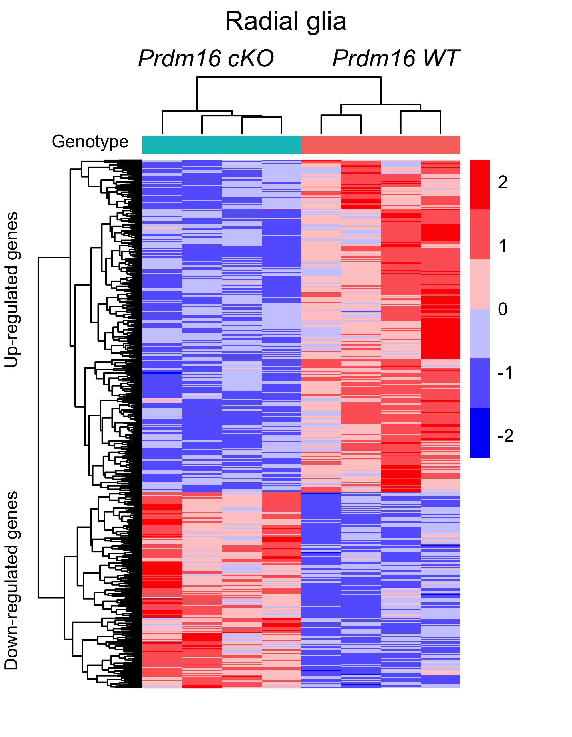
Finally, we want to export the image so that it will display properly in our final figure.
# Save image
ggsave(filename = "results/heatmap_figure.png",
       plot = heatmap_figure,
       units = "in",
       width = 4,
       height = 5.15,
       dpi = 500)