Approximate time: 20 minutes

Learning Objectives

• Create a custom theme to facilitate consistency between plots

Consistent formatting using custom themes

When publishing, it is helpful to ensure plots have consistent formatting. To do this we can create a custom function with our preferences for the theme. Remember the structure of a function is:

name_of_function <- function(arguments) {
    statements or code that does something
}

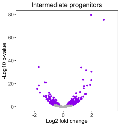
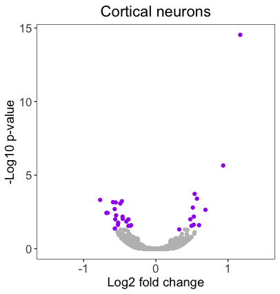
We need to create two additional volcano plots that should look very similar to our original ‘Radial glia’ plot for the ‘Intermediate progenitors’ and the ‘Cortical neurons’. The code for the original plot is displayed below:

# Volcano plot for radial glia
ggplot(results) +
  geom_point(aes(x = pax6_log2FoldChange, 
                 y = -log10(pax6_padj), 
                 color = pax6_threshold))  +
  ggtitle("Radial glia") +
  theme_bw() +
  theme(axis.title = element_text(size = rel(1.25)),
        axis.text = element_text(size = rel(1.15))) +
  theme(plot.title = element_text(size = rel(1.5))) +
  theme(legend.position = "none") +
  theme(panel.grid = element_blank()) +
  theme(plot.title=element_text(hjust=0.5)) +
  scale_color_manual(values = c("grey", "purple")) +
  scale_x_continuous(name = "Log2 fold change", 
                     limits = c(-3, 3.5)) +
  scale_y_continuous(name = "-Log10 p-value")

To ensure consistency between our volcano plots, we want our volcano plot themes to be consistent between all 3 plots. We can do this by extracting the theme() layers (shown below) and applying them to every plot:

# DO NOT RUN
theme_bw() +
  theme(axis.title = element_text(size = rel(1.25)),
        axis.text = element_text(size = rel(1.15))) +
  theme(plot.title = element_text(size = rel(1.5))) +
  theme(legend.position = "none") +
  theme(panel.grid = element_blank()) +
  theme(plot.title=element_text(hjust=0.5))

You can also combine multiple arguments within the same theme() function:

# DO NOT RUN
theme_bw() +
  theme(axis.title = element_text(size = rel(1.25)),
        axis.text = element_text(size = rel(1.15)),
        plot.title = element_text(size = rel(1.5),
                                  hjust = 0.5),
        panel.grid = element_blank(),
        legend.position = "none")

Creating a function that represents these thematic changes is simple; we can just put the above code inside the {}:

# Creating function for personal theme to apply to all plots
personal_theme <- function(){ 
  theme_bw() +
  theme(axis.title = element_text(size = rel(1.25)),
        axis.text = element_text(size = rel(1.15)),
        plot.title = element_text(size = rel(1.5),
                                  hjust = 0.5),
        panel.grid = element_blank(),
        legend.position = "none")
}

Now to run our personal theme with any plot, we can use this function in place of all of the lines of code associated with theme() layers:

# Creating volcano plot using the 'personal_theme()` function
ggplot(results) +
  geom_point(aes(x = pax6_log2FoldChange, 
                 y = -log10(pax6_padj), 
                 color = pax6_threshold)) +
  personal_theme() +
  ggtitle("Radial glia") +
  scale_color_manual(values = c("grey", "purple")) +
  scale_x_continuous(name = "Log2 fold change", 
                     limits = c(-3, 3.5)) +
  scale_y_continuous(name = "-Log10 p-value")

Now that we have the final volcano plot, let’s save it to a variable, which we can use downstream to add our annotations.

# Save volcano plot to a variable
volcano_RG <- ggplot(results) +
  geom_point(aes(x = pax6_log2FoldChange, 
                 y = -log10(pax6_padj), 
                 color = pax6_threshold)) +
  personal_theme() +
  ggtitle("Radial glia") +
  scale_color_manual(values = c("grey", "purple")) +
  scale_x_continuous(name = "Log2 fold change", 
                     limits = c(-3, 3.5)) +
  scale_y_continuous(name = "-Log10 p-value")

---

Exercise

Using your personal_theme(), create volcano plots for the ‘Intermediate progenitors’ and the ‘Cortical neurons’ by using the tbr2_ and neg_ columns from the results data frame, respectively. Save the plots to the variables volcano_IP and volcano_neu.

---

This lesson has been developed by members of the teaching team at the Harvard Chan Bioinformatics Core (HBC). These are open access materials distributed under the terms of the Creative Commons Attribution license (CC BY 4.0), which permits unrestricted use, distribution, and reproduction in any medium, provided the original author and source are credited.