Learning Objectives
- What is RMarkdown?
- What are the uses of RMarkdown
- Creating html reports using knitr
Generating research analysis reports with RMarkdown
For any experimental analysis, it is critical to keep detailed notes for the future reproduction of the experiment and for the interpretation of results. For laboratory work, lab notebooks allow us to organize our methods, results, and conclusions to allow for future retrieval and reproduction. Computational analysis requires the same diligence, but it is often easy to forget to completely document the analysis and/or interpret the results in a transparent fashion.
For analyses within R, RStudio helps facilitate reproducible research with the use of R scripts, which can be used to save all code used to perform a particular analysis. However, we often don’t save the version of the tools we use in a script, nor do we include or interpret the results of the analyses within the script.
Wouldn’t it be nice to be able to save/share the code with collaborators along with tables, figures, and text describing the interpretation in a single, cleaned up report file?
The knitr package, developed by Yihui Xie, is designed to generate reports within RStudio. It enables dynamic generation of multiple file formats from an RMarkdown file, including HTML and PDF documents. Knit report generation is now integrated into RStudio, and can be accessed using the GUI or console.
In this workshop we will become familiar with both knitr and the RMarkdown language. Before we delve into the details we will start with an activity to show you what an RMarkdown file looks like and the HTML report once you have used the knit() function.
Activity 1
- Create a new project in a new directory called
rmd_workshop - Download this RMarkdown file and save within the
rmd_workshopproject directory - Download and uncompress this data folder within the project directory
- Open the .rmd file in RStudio
- knit the markdown
Note: If you run into error when kniting the markdown, make sure your data structure is set properly as below:
- The
datafolder is in the same directory asworkshop-example.rmdfile - Two files (
counts.rpkm.csvandmouse_exp_design.csv) are located inside thedatafolder
- The
RMarkdown basics
The Markdown language for formatting plain text format has been adopted by many different coding groups, and some have added their own “flavours”. RStudio implements something called “R-flavoured markdown” or “RMarkdown” which has really nice features for text and code formatting as described below.
As RMarkdown grows as an acceptable reproducible manuscript format, using knitr to generate a report summary is becoming common practice.
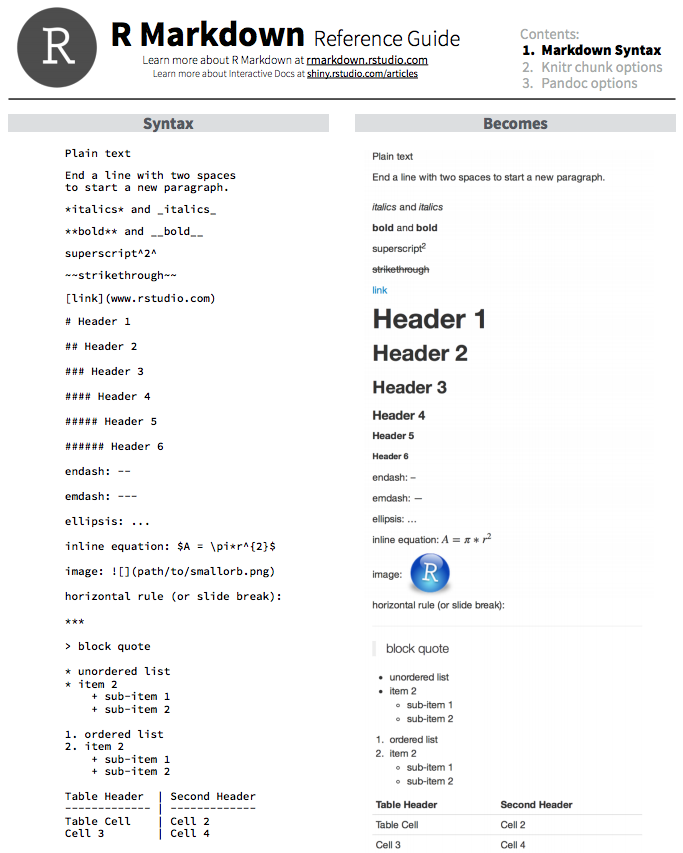
Text
The syntax to format the text portion of the report is relatively easy. You can easily get text that is bolded, italicized, bolded & italicized. You can create “headers” and “sub-headers” by placing an “#” or “##” and so on in front of a line of text, generate numbered and bulleted lists, add hyperlinks to words or phrases, and so on.
Let’s take a look at the syntax of how to do this in RMarkdown before we move on to formatting and adding code chunks:
You can also get more information about text formatting here and here.
Code chunks
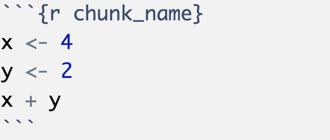
The basic idea is that you can write your analysis workflow in plain text and intersperse chunks of R code delimited with a special marker (```). Backticks (`) commonly indicate code and are also used for formatting on GitHub.
Each individual code chunk should be given a unique name. knitr isn’t very picky how you name the code chunks, but we recommend using snake_case for the names whenever possible.
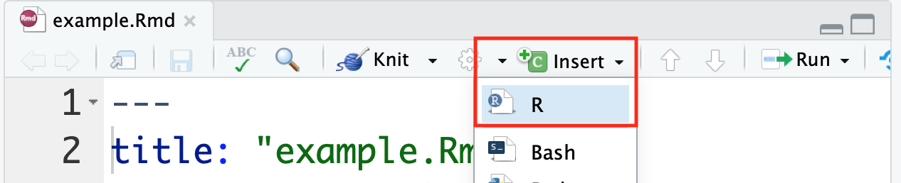
There is a handy Insert button within RStudio that allows for the insertion of an empty R chunk if desired.
Additionally, you can write inline R code enclosed by single backticks (`) containing a lowercase r (like ``` code chunks). This allows for variable returns outside of code chunks, and is extremely useful for making report text more dynamic. For example, you can print the current date inline within the report with this syntax: `r Sys.Date()` (no spaces).
As the final chunk in your analysis, it is recommended to run the sessionInfo() function. This function will output the R version and the versions of all libraries loaded in the R environment. The versions of the tools used is important information for reproduction of your analysis in the future.
Activity 2
- Add a new section header in the same size as the “Project details” header at the end
- Next, add a new code chunk below it to display the output of
sessionInfo() - Modify the
AuthorandTitleparameters at the top of the script - knit the markdown
Options for code chunks
The knitr package provides a lot of customization options for code chunks, which are written in the form of tag=value.
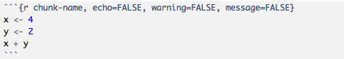
There is a comprehensive list of all the options available, however when starting out this can be overwhelming. Here, we provide a short list of some options commonly use in chunks:
echo = TRUE: whether to include R source code in the final document. If echo = FALSE, R source code will not be written into the final document. But the code is still evaluated and its output will be included in the final documenteval = TRUE: whether to evaluate/execute the codeinclude = TRUE: whether to include R source code and its output in the final document. If include = FALSE, nothing (R source code and its output) will be written into the final document. But the code is still evaluated and plot files are generated if there are any plots in the chunkwarning = TRUE: whether to preserve warnings in the output like we run R code in a terminal (if FALSE, all warnings will be printed in the console instead of the output document)message = TRUE: whether to preserve messages emitted by message() (similar to warning)results = "asis": output as-is, i.e., write raw results from R into the output document instead of LaTeX-formatted output. Another useful option for this option is “hide”, which will hide the results, or all normal R output
The setup chunk
The setup chunk is a special knitr chunk that should be placed at the start of the document. We recommend storing all library() loads required for the script and other load() requests for external files here. In our RMarkdown templates, such as the bcbioRnaseq differential expression template, we store all the user-defined parameters in the setup chunk that are required for successful knitting.
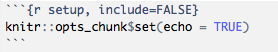
Global options
knitr allows for global options to be set on all chunks in an RMarkdown file. These are options that should be placed inside your setup chunk at the top of your RMarkdown document. These will be the default options used for all the code chunks in the document, however they can be modified for each code chunk.
opts_chunk$set(
    autodep = TRUE,
    cache = TRUE,
    cache.lazy = TRUE,
    dev = c("png", "pdf", "svg"),
    error = TRUE,
    fig.height = 6,
    fig.retina = 2,
    fig.width = 6,
    highlight = TRUE,
    message = FALSE,
    prompt = TRUE,
    tidy = TRUE,
    warning = FALSE)
An additional cool trick is that you can save opts_chunk$set settings in ~/.Rprofile and these knitr options will apply to all of your RMarkdown documents, and not just the one.
Activity 3
- Only some of the code chunks have names; go through and add names to the unnamed code chunks.
- For the code chunk named
data-orderingdo the following:- First, add a new line of code that displays a small part of the newly created
data_ordereddata frame usinghead() - Next, modify the options for (
{r data-ordering}) such that the output from the new line of code shows up in the report, but not the code
- First, add a new line of code that displays a small part of the newly created
- Without removing the last code chunk (for boxplot) from the Rmd file, modify its options such that neither the code nor its output appear in the report
- knit the markdown
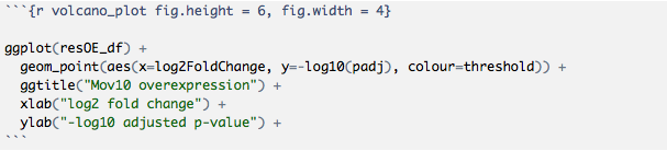
Figures
A neat feature of knitr is how much simpler it makes generating figures. You can simply return a plot in a chunk, and knitr will automatically write the files to disk, in an organized subfolder. By specifying options in the setup chunk, you can have R automatically save your plots in multiple file formats at once, including PNG, PDF, and SVG. A single chunk can support multiple plots, and they will be arranged in squares below the chunk in RStudio.
There are also a few options commonly used for plots to easily resize the figures in the final report. You can specify the height and width of the figure when setting up the code chunk.
Tables
knitr includes a simple but powerful function for generating stylish tables in a knit report named kable(). Here’s an example using R’s built-in mtcars dataset:
help("kable", "knitr")
mtcars %>%
    head %>%
    kable
| mpg | cyl | disp | hp | drat | wt | qsec | vs | am | gear | carb | |
|---|---|---|---|---|---|---|---|---|---|---|---|
| Mazda RX4 | 21.0 | 6 | 160 | 110 | 3.90 | 2.620 | 16.46 | 0 | 1 | 4 | 4 |
| Mazda RX4 Wag | 21.0 | 6 | 160 | 110 | 3.90 | 2.875 | 17.02 | 0 | 1 | 4 | 4 |
| Datsun 710 | 22.8 | 4 | 108 | 93 | 3.85 | 2.320 | 18.61 | 1 | 1 | 4 | 1 |
| Hornet 4 Drive | 21.4 | 6 | 258 | 110 | 3.08 | 3.215 | 19.44 | 1 | 0 | 3 | 1 |
| Hornet Sportabout | 18.7 | 8 | 360 | 175 | 3.15 | 3.440 | 17.02 | 0 | 0 | 3 | 2 |
| Valiant | 18.1 | 6 | 225 | 105 | 2.76 | 3.460 | 20.22 | 1 | 0 | 3 | 1 |
There are some other functions that allow for more powerful customization of tables, including pander::pander() and xtable::xtable(), but the simplicity and cross-platform reliability of knitr::kable() makes it an easy pick.
Generating the report
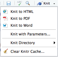
Once we’ve finished creating an RMarkdown file containing code chunks, we finally need to knit the report. You can knit it by using the knit() function, or by just clicking on “knit” in the panel above the script as we had done in our first activity in this lesson.
When executing knit() on a document, by default this will generate an HTML report. If you would prefer a different document format, this can be specified in the YAML header with the output: parameter. You can also click on the button in the panel above the script and click on “Knit” to get the various options as shown below:
Note: PDF rendering is sometimes problematic, especially when running R remotely, like on the cluster (Odyssey or O2). If you run into problems, it’s likely an issue related to pandoc.
The RStudio cheatsheet for Rmarkdown is quite daunting, but includes more advanced Rmarkdown options that may be helpful as you become familiar with report generation, including options for adding interactive plots RShiny.
Activity 4
- Download the linked R script
- Download the linked RData object by right-clicking and save to
datafolder. - Transform the R script into a new RMarkdown file with the following specifications:
- Create an R chunk for all code underneath each
#comment in the original R script - Comment on the plots (you may have to run the code from the R script to see the plots first)
- Add a floating table of contents
- Create an R chunk for all code underneath each
- knit the markdown
Note1: output formats
RStudio supports a number of formats, each with their own customization options. Consult their website for more details.
The
knit()command works great if you only need to generate a single document format. RMarkdown also supports a more advanced function namedrmarkdown::render(), allows for output of multiple document formats. To accomplish this, we recommend saving a special file named_output.yamlin your project root. Here’s an example from our bcbioRnaseq package:rmarkdown::html_document: code_folding: hide df_print: kable highlight: pygments number_sections: false toc: true rmarkdown::pdf_document: number_sections: false toc: true toc_depth: 1
Note2: working directory behavior
knitr redefines the working directory of an RMarkdown file in a manner that can be confusing. If you’re working in RStudio with an RMarkdown file that is not at the same location as the current R working directory (
getwd()), you can run into problems with broken file paths. Make sure that any paths to files specified in the RMarkdown document is relative to its location, and not your current working directory.A simple way to make sure that the paths are not an issue is by creating an R project for the analysis, and saving all RMarkdown files at the top level and referring to the data and output files within the project directory. This will prevent unexpected problems related to this behavior.
Additional resources
This lesson has been developed by members of the teaching team and Michael J. Steinbaugh at the Harvard Chan Bioinformatics Core (HBC). These are open access materials distributed under the terms of the Creative Commons Attribution license (CC BY 4.0), which permits unrestricted use, distribution, and reproduction in any medium, provided the original author and source are credited.