Comprehensive practical - answer key

Creating vectors/factors and data frames

We are performing RNA-Seq on cancer samples being treated with three different types of treatment (A, B, and P). You have 12 samples total, with 4 replicates per treatment. Write the R code you would use to construct your metadata table as described below.

Create the vectors/factors for each column (Hint: you can type out each vector/factor, or if you want the process go faster try exploring the rep() function).

   sex <- c("M", "F",...) # saved vectors/factors as variables and used c() or 
   sex <- rep(c("M", "F"), times = 6)
   stage <- rep(c("I", "II", "II"), times = 4)
   treatment <- rep(c("A", "B", "P"), each = 4)
   myc <- c(2343,457,4593,9035,3450,3524,958,1053,8674,3424,463,5105)

Put them together into a dataframe called meta.

  meta <- data.frame(sex, stage, treatment, myc) # used data.frame() to create the table

Use the rownames() function to assign row names to the dataframe (Hint: you can type out the row names as a vector, or if you want the process go faster try exploring the paste() function).

  rownames(meta) <- c("sample1", "sample2",... , "sample12") # or use:
     
  rownames(meta) <- paste("sample", 1:12, sep="")

Your finished metadata table should have information for the variables sex, stage, treatment, and myc levels:

	sex	stage	treatment	myc
sample1	M	I	A	2343
sample2	F	II	A	457
sample3	M	II	A	4593
sample4	F	I	A	9035
sample5	M	II	B	3450
sample6	F	II	B	3524
sample7	M	I	B	958
sample8	F	II	B	1053
sample9	M	II	P	8674
sample10	F	I	P	3424
sample11	M	II	P	463
sample12	F	II	P	5105

Subsetting vectors/factors and dataframes

Using the meta data frame from question #1, write out the R code you would use to perform the following operations (questions DO NOT build upon each other):
- return only the treatment and sex columns using []:
```
  meta[ , c(1,3)]
```
- return the treatment values for samples 5, 7, 9, and 10 using []:
```
  meta[c(5,7,9,10), 3]
```
- remove the treatment column from the dataset using []:
```
  meta[, -3]
```
- remove samples 7, 8 and 9 from the dataset using []:
```
  meta[-7:-9, ]
```
- keep only samples 1-6 using []:
```
  meta[1:6, ]
```
- output a data frame with a column called pre_treatment as the first column with the values T, F, F, F, T, T, F, T, F, F, T, T (Hint: use data.frame or cbind()):
```
  pre_treatment <- c(T, F, F, F, T, T, F, T, F, F, T, T)
     
  cbind(pre_treatment, meta)
```
- change the names of the columns to: “A”, “B”, “C”, “D”:
```
  colnames(meta) <- c("A", "B", "C", "D")
```

Extracting components from lists

Create a new list, list_three with three components, the pre_treatment vector, the dataframe meta, and vector stage. Use this list to answer the questions below . list_three has the following structure (NOTE: the components of this list are not currently named):
```
   [[1]]
   [1]   4.6  3000.0 50000.0 

   [[2]]
          species  glengths 
     1    ecoli    4.6
     2    human    3000.0
     3    corn     50000.0

   [[3]]
   [1] 8
```

  list_three <- list(pre_treatment, meta, stage)

Write out the R code you would use to perform the following operations (questions DO NOT build upon each other):

return the second component of the list:

 list_three[[2]]

return 2343 from the second component of the list:

 list_three[[2]][1,4]
  #or
 comp2 <- list_three[[2]]
 comp2[1,4]

return all “I” values from the third component:

 list_three[[3]][c(1,4,7,10)]
  #or 
 comp3 <- list_three[[3]]
 comp3[c(1,4,7,10)]

give the components of the list the following names: “pre_treatment”, “meta”, “stage”:

 names(list_three) <- c("pre_treatment", "meta", "stage")

Creating figures with ggplot2

plot_image

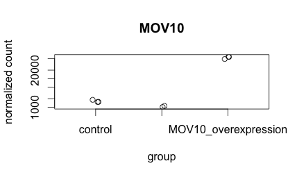
Create the same plot as above using ggplot2 using the provided metadata and counts datasets. The metadata table describes an experiment that you have setup for RNA-seq analysis, while the associated count matrix gives the normalized counts for each sample for every gene. Download the count matrix and metadata using the links provided.

Follow the instructions below to build your plot. Write the code you used and provide the final image.
- Read in the metadata file (“Mov10_full_meta.txt”) to a variable called meta using the read.delim() function. Be sure to specify the row names are in column 1 and the delimiter/column separator is a tab (“/t”).
  
  counts_meta <- read.delim("data/Mov10_full_meta.txt", sep="\t", row.names=1)
- Read in the count matrix file (“normalized_counts.txt”) to a variable called data using the read.delim() function and specifying there are row names in column 1 and the tab delimiter.
  
  data <- read.delim("data/normalized_counts.txt", sep="\t", row.names=1)
- Create a variable called expression that contains the normalized count values from the row in data that corresponds to the MOV10 gene.
```
  expression <- data["MOV10", ]
```
- Check the class of expression. data.frame
Convert this to a numeric vector using as.numeric(expression)
```
  class(expression)
     
  expression <- as.numeric(expression)
     
  class(expression)
     
```
- Bind that vector to your metadata data frame (counts_meta) and call the new data frame df.
```
  df <- cbind(counts_meta, expression) #or
     
  df <- data.frame(counts_meta, expression)
```
- Create a ggplot by constructing the plot line by line:
  - Initialize a ggplot with your df as input.
  - Add the geom_jitter() geometric object with the required aesthetics
  - Color the points based on sampletype
  - Add the theme_bw() layer
  - Add the title “Expression of MOV10” to the plot
  - Change the x-axis label to be blank
  - Change the y-axis label to “Normalized counts”
  - Using theme() change the following properties of the plot:
    - Remove the legend (Hint: use ?theme help and scroll down to legend.position)
    - Change the plot title size to 1.5x the default and center align
    - Change the axis title to 1.5x the default size
    - Change the size of the axis text only on the y-axis to 1.25x the default size
    - Rotate the x-axis text to 45 degrees using axis.text.x=element_text(angle=45, hjust=1)
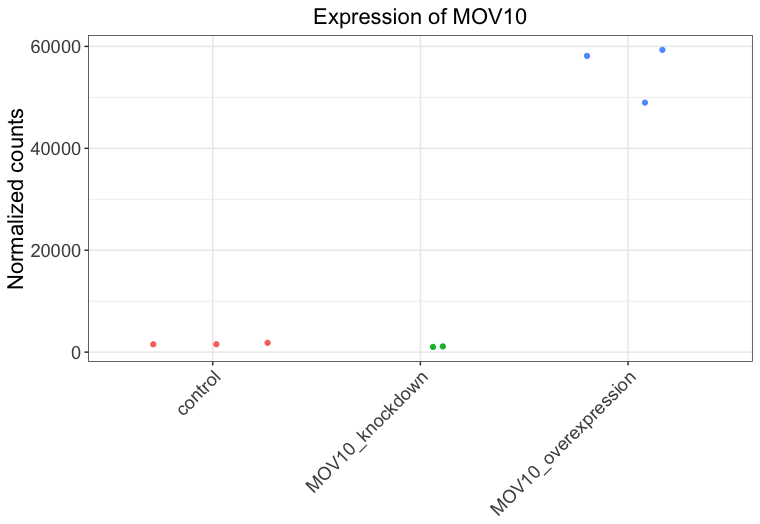
```
   ggplot(df) +
     geom_jitter(aes(x= sampletype, y= expression, color = sampletype)) +
     theme_bw() +
     ggtitle("Expression of MOV10") +
     xlab(NULL) +
     ylab("Normalized counts") +
     theme(legend.position = "none",
           plot.title=element_text(hjust=0.5, size=rel(1.5)),
           axis.text=element_text(size=rel(1.25)),
           axis.title=element_text(size=rel(1.5)),
           axis.text.x=element_text(angle=45, hjust=1))
```
Save the plot as a PDF to the figures directory.

```r pdf(“figures/name_of_plot.pdf”)

ggplot(df) + geom_jitter(aes(x= sampletype, y= expression, color = sampletype)) + theme_bw() + ggtitle(“Expression of MOV10”) + xlab(NULL) + ylab(“Normalized counts”) + theme(legend.position = “none”, plot.title=element_text(hjust=0.5, size=rel(1.5)), axis.text=element_text(size=rel(1.25)), axis.title=element_text(size=rel(1.5)), axis.text.x=element_text(angle=45, hjust=1))

dev.off()

Packages and installations

Install the tidyverse R package from the CRAN repository and load the library.

  install.packages("tidyverse")
  library(tidyverse)

Install the biomaRt R package from the Bioconductor repository and load the library.

  #install.packages("BiocManager")
  library(BiocManager)
  install("biomaRt")
  library(biomaRt)

Building on the basics

The Tidyverse suite of integrated packages are R packages designed to work together to make common data science operations more user friendly. The packages have functions for data wrangling, tidying, reading/writing, parsing, and visualizing, among others.

Using this tutorial, explore some of the functionality for reading in and wrangling data with the readr and dplyr packages, which were installed when you installed the tidyverse suite in the previous section.
Turn the meta data frame from question #1 of the “Creating vectors/factors and data frames” section above into a tibble called meta_tb. (Hint: Be sure to turn the rownames into a column before changing it into a tibble.)

  meta_tb <- meta %>%
  rownames_to_column(var = "sample") %>%
  as_tibble()

Using meta_tb, write out the R code you would use to rename the columns back to sex, stage, treatment, and myc using rename(). Save back (overwrite) to the meta_tb variable.

  meta_tb <- meta_tb %>%
  rename(sex = A,
         stage = B,
         treatment = C,
         myc = D)

Using meta_tb, write out the R code you would use to perform the following operations (questions DO NOT build upon each other):
- use filter() to return all data for those samples receiving treatment P.
```
 meta_tb %>%
 filter(treatment == "P")
```
- use filter()/select() to return only the stage and treatment columns for those samples with myc > 5000.
```
 meta_tb %>%
 filter(myc > 5000) %>%
 dplyr::select(stage, treatment)
```
- use arrange() to arrange the rows by myc in descending order.
```
 meta_tb %>%
 arrange(desc(myc))
```

Write meta_tb to file using the write_delim() function.

 write_delim(meta_tb, 
        file = "results/metadata_myc_by_stage_sex.csv", 
        delim = ",")