Approximate time: 30 min
Learning Objectives
- Reading data into R
- Inspecting data structures
- Using indexes to select data from vectors and data frames
Reading data into R
Regardless of the specific analysis in R we are performing, we usually need to bring data in for the analysis. The function in R we use will depend on the type of data file we are bringing in (e.g. text, Stata, SPSS, SAS, Excel, etc.) and how the data in that file are separated, or delimited. The table below lists functions that can be used to import data from common file formats.
| Data type | Extension | Function | Package |
|---|---|---|---|
| Comma separated values | csv | read.csv() |
utils (default) |
read_csv() |
readr (tidyverse) | ||
| Tab separated values | tsv | read_tsv() |
readr |
| Other delimited formats | txt | read.table() |
utils |
read_table() |
readr | ||
read_delim() |
readr | ||
| Stata version 13-14 | dta | readdta() |
haven |
| Stata version 7-12 | dta | read.dta() |
foreign |
| SPSS | sav | read.spss() |
foreign |
| SAS | sas7bdat | read.sas7bdat() |
sas7bdat |
| Excel | xlsx, xls | read_excel() |
readxl (tidyverse) |
For example, if we have text file separated by commas (comma-separated values), we could use the function read.csv. However, if the data are separated by a different delimiter in a text file, we could use the generic read.table function and specify the delimiter as an argument in the function.
When working with genomic data, we often have a metadata file containing information on each sample in our dataset. Let’s bring in the metadata file using the read.csv function. Check the arguments for the function to get an idea of the function options:
?read.csv
The read.csv function has one required argument and several options that can be specified. The mandatory argument is a path to the file and filename, which in our case is data/mouse_exp_design.csv. We will put the function to the right of the assignment operator, meaning that any output will be saved as the variable name provided on the left.
metadata <- read.csv(file="data/mouse_exp_design.csv")
Note: By default,
read.csvconverts (= coerces) columns that contain characters (i.e., text) into thefactordata type. Depending on what you want to do with the data, you may want to keep these columns ascharacter. To do so,read.csv()andread.table()have an argument calledstringsAsFactorswhich can be set toFALSE.
Inspecting data structures
There are a wide selection of base functions in R that are useful for inspecting your data and summarizing it. Let’s use the metadata file that we created to test out data inspection functions.
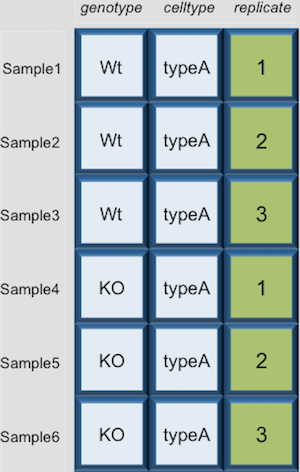
Take a look at the dataframe by typing out the variable name metadata and pressing return; the variable contains information describing the samples in our study. Each row holds information for a single sample, and the columns contain categorical information about the sample genotype(WT or KO), celltype (typeA or typeB), and replicate number (1,2, or 3).
metadata

          genotype celltype replicate
sample1        Wt    typeA		1
sample2        Wt    typeA		2
sample3        Wt    typeA		3
sample4        KO    typeA		1
sample5        KO    typeA		2
sample6        KO    typeA		3
sample7        Wt    typeB		1
sample8        Wt    typeB		2
sample9        Wt    typeB		3
sample10       KO    typeB		1
sample11       KO    typeB		2
sample12       KO    typeB		3
Suppose we had a larger file, we might not want to display all the contents in the console. Instead we could check the top (the first 6 lines) of this data.frame using the function head():
head(metadata)
Previously, we had mentioned that character values get converted to factors by default using data.frame. One way to assess this change would be to use the __str__ucture function. You will get specific details on each column:
str(metadata)

'data.frame':	12 obs. of  3 variables:
 $ genotype : Factor w/ 2 levels "KO","Wt": 2 2 2 1 1 1 2 2 2 1 ...
 $ celltype : Factor w/ 2 levels "typeA","typeB": 1 1 1 1 1 1 2 2 2 2 ...
 $ replicate: num  1 2 3 1 2 3 1 2 3 1 ...
As you can see, the columns genotype and celltype are of the factor class, whereas the replicate column has been interpreted as integer data type.
You can also get this information from the “Environment” tab in RStudio.
List of functions for data inspection
We already saw how the functions head() and str() can be useful to check the
content and the structure of a data.frame. Here is a non-exhaustive list of
functions to get a sense of the content/structure of data.
- All data structures - content display:
str(): compact display of data contents (env.)class(): data type (e.g. character, numeric, etc.) of vectors and data structure of dataframes, matrices, and lists.summary(): detailed display, including descriptive statistics, frequencieshead(): will print the beginning entries for the variabletail(): will print the end entries for the variable
- Vector and factor variables:
length(): returns the number of elements in the vector or factor
- Dataframe and matrix variables:
dim(): returns dimensions of the datasetnrow(): returns the number of rows in the datasetncol(): returns the number of columns in the datasetrownames(): returns the row names in the datasetcolnames(): returns the column names in the dataset
Selecting data using indexes and sequences
When analyzing data, we often want to partition the data so that we are only working with selected columns or rows. A data frame or data matrix is simply a collection of vectors combined together. So let’s begin with vectors and how to access different elements, and then extend those concepts to dataframes.
Vectors
Selecting using indexes
If we want to extract one or several values from a vector, we must provide one or several indexes using square brackets [ ] syntax. The index represents the element number within a vector (or the compartment number, if you think of the bucket analogy). R indexes start at 1. Programming languages like Fortran, MATLAB, and R start counting at 1, because that’s what human beings typically do. Languages in the C family (including C++, Java, Perl, and Python) count from 0 because that’s simpler for computers to do.
Let’s start by creating a vector called age:
age <- c(15, 22, 45, 52, 73, 81)
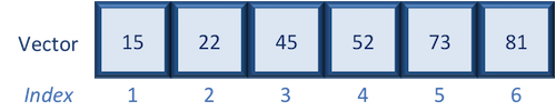
Suppose we only wanted the fifth value of this vector, we would use the following syntax:
age[5]
If we wanted all values except the fifth value of this vector, we would use the following:
age[-5]
If we wanted to select more than one element we would still use the square bracket syntax, but rather than using a single value we would pass in a vector of several index values:
idx <- c(3,5,6) # create vector of the elements of interest
age[idx]
To select a sequence of continuous values from a vector, we would use : which is a special function that creates numeric vectors of integer in increasing or decreasing order. Let’s select the first four values from age:
age[1:4]
Alternatively, if you wanted the reverse could try 4:1 for instance, and see what is returned.
NOTE: Selection of values can also be performed using logical expressions. Logical operators include greater than (>), less than (<), and equal to (==). We can use logical expressions to determine whether a particular condition is true or false. Then, subset out the TRUE values:
age[age > 50][1] 52 73 81More details about using logical expressions to subset data can be found here
Dataframes
Dataframes (and matrices) have 2 dimensions (rows and columns), so if we want to select some specific data from it we need to specify the “coordinates” we want from it. We use the same square bracket notation but rather than providing a single index, there are two indexes required. Within the square bracket, row numbers come first followed by column numbers (and the two are separated by a comma). Let’s explore the metadata dataframe, shown below are the first six samples:
For example:
metadata[1, 1]   # element from the first row in the first column of the data frame
metadata[1, 3]   # element from the first row in the 3rd column
Now if you only wanted to select based on rows, you would provide the index for the rows and leave the columns index blank. The key here is to include the comma, to let R know that you are accessing a 2-dimensional data structure:
metadata[3, ] # vector containing all elements in the 3rd row
If you were selecting specific columns from the data frame - the rows are left blank:
metadata[ , 3] # vector containing all elements in the 3rd column
Just like with vectors, you can select multiple rows and columns at a time. Within the square brackets, you need to provide a vector of the desired values:
metadata[ , 1:2] # dataframe containing first two columns
metadata[c(1,3,6), ] # dataframe containing first, third and sixth rows
For larger datasets, it can be tricky to remember the column number that corresponds to a particular variable. (Is celltype in column 1 or 2? oh, right… they are in column 1). In some cases, the column number for a variable can change if the script you are using adds or removes columns. It’s therefore often better to use column names to refer to a particular variable, and it makes your code easier to read and your intentions clearer.
metadata[1:3 , "celltype"] # elements of the celltype column corresponding to the first three samples
You can do operations on a particular column, by selecting it using the $ sign. In this case, the entire column is a vector. For instance, to extract all the gentotypes from our dataset, we can use:
metadata$genotype
You can use names(metadata) or colnames(metadata) to remind yourself of the column names. We can then supply index values to select specific values from that vector. For example, if we wanted the genotype information for the first five samples in metadata:
colnames(metadata)

metadata$genotype[1:5]
The $ allows you to select a single column by name. To select multiple columns by name, you need to concatenate a vector of strings that correspond to column names:
metadata[, c("genotype", "celltype")]
          genotype celltype
sample1        Wt    typeA
sample2        Wt    typeA
sample3        Wt    typeA
sample4        KO    typeA
sample5        KO    typeA
sample6        KO    typeA
sample7        Wt    typeB
sample8        Wt    typeB
sample9        Wt    typeB
sample10       KO    typeB
sample11       KO    typeB
sample12       KO    typeB
While there is no equivalent $ syntax to select a row by name, you can select specific rows using the row names. To remember the names of the rows, you can use the rownames() function:
rownames(metadata)

metadata[c("sample10", "sample12"),]
Subsetting data
Another way of partitioning dataframes is using the subset() function to return the rows of the dataframe for which the logical expression is TRUE. Allowing us to the subset the data in a single step. The syntax for the subset() function is:
subset(dataframe, column_name == "value") # Any logical expression could replace the `== "value"`
For example, we can look at the samples of a specific celltype “typeA”:
subset(metadata, celltype == "typeA")
         genotype celltype replicate
sample1       Wt    typeA         1
sample2       Wt    typeA         2
sample3       Wt    typeA         3
sample4       KO    typeA         1
sample5       KO    typeA         2
sample6       KO    typeA         3
We can also use the subset function with the other logical operators in R. For example, suppose we wanted to subset to keep only the WT samples from the typeA celltype.
subset(metadata, celltype == "typeA" & genotype == "Wt")
        genotype celltype replicate
sample1       Wt    typeA         1
sample2       Wt    typeA         2
sample3       Wt    typeA         3
Alternatively, we could try looking at only the first two replicates of each sample set. Here, we can use the less than operator since replicate is currently a numeric vector. Adding in the argument select allows us to specify which columns to keep, with the syntax:
subset(dataframe, column_name == "value", select = "name of column(s) to return")
Which columns are left?
sub_meta <- subset(metadata, replicate < 3, select = c('genotype', 'celltype'))
Lists
Selecting components from a list requires a slightly different notation, even though in theory a list is a vector (that contains multiple data structures). To select a specific component of a list, you need to use double bracket notation [[]]. Let’s use the list1 that we created previously, and index the second component:
list1[[2]]
What do you see printed to the console? Using the double bracket notation is useful for accessing the individual components whilst preserving the original data structure. When creating this list we know we had originally stored a dataframe in the second component. With the class function we can check if that is what we retrieve:
comp2 <- list1[[2]]
class(comp2)
Writing to file
Everything we have done so far has only modified the data in R; the files have remained unchanged. Whenever we want to save our datasets to file, we need to use a write function in R.
To write our matrix to file in comma separated format (.csv), we can use the write.csv function. There are two required arguments: the variable name of the data structure you are exporting, and the path and filename that you are exporting to. By default the delimiter is set, and columns will be separated by a comma:
write.csv(sub_meta, file="data/subset_meta.csv")
Similar to reading in data, there are a wide variety of functions available allowing you to export data in specific formats. Another commonly used function is write.table, which allows you to specify the delimiter you wish to use. This function is commonly used to create tab-delimited files.
NOTE:
Sometimes when writing a data frame with row names to file, the column names will align starting with the row names column. To avoid this, you can include the argument
col.names = NAwhen writing to file to ensure all of the column names line up with the correct column values.
Writing a vector of values to file requires a different function than the functions available for writing dataframes. You can use
write()to save a vector of values to file. For example:
write(glengths, file="genome_lengths.txt", ncolumns=1)
An R package for data science
The methods presented above are using base R functions for data manipulation. For more advanced R users, the
tidyversepackage, which contains a suite of packages providing tools for the most common data science tasks.
This lesson has been developed by members of the teaching team at the Harvard Chan Bioinformatics Core (HBC). These are open access materials distributed under the terms of the Creative Commons Attribution license (CC BY 4.0), which permits unrestricted use, distribution, and reproduction in any medium, provided the original author and source are credited.
- The materials used in this lesson is adapted from work that is Copyright © Data Carpentry (http://datacarpentry.org/). All Data Carpentry instructional material is made available under the Creative Commons Attribution license (CC BY 4.0).