Set-up DESeq2 analysis - Answer Key

Exercise 1

1. Use the dds_APC object to compute the rlog transformed counts for the Pdgfr α+ APCs.

# Transform counts for data visualization
rld_APC <- rlog(dds_APC, blind = TRUE)

2. Create a PCA plot for the Pdgfr α+ APCs, coloring points by condition. Do samples segregate by condition? Is there more or less variability within group than observed with the VSM cells?

# Plot PCA
plotPCA(rld_APC, intgroup = c("condition")) + theme_classic()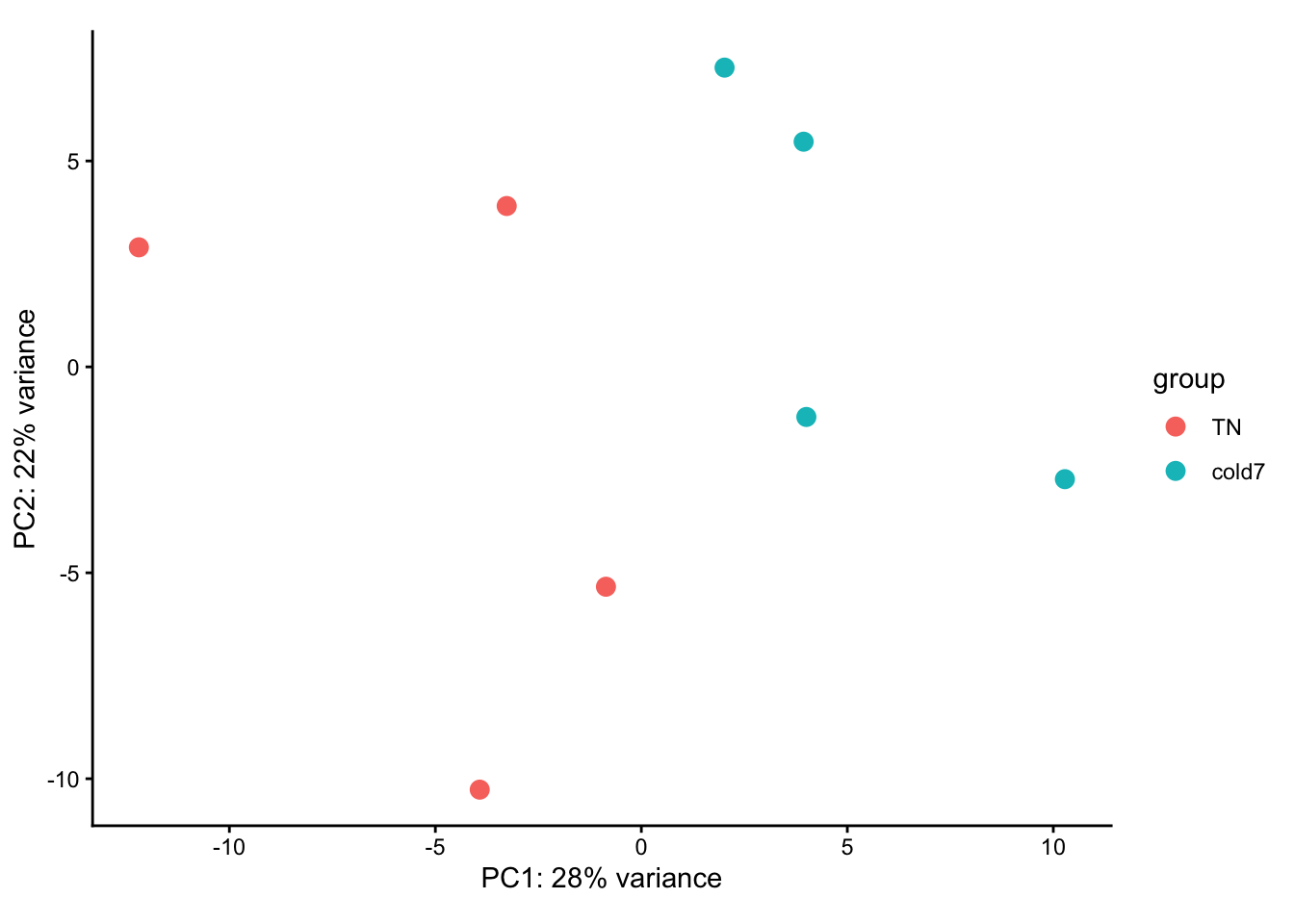

3. Evaluate the sample similarity using a correlation heatmap. How does this compare with the trends observed in the PCA plot?

# Calculate sample correlation
rld_APC_mat <- assay(rld_APC)
rld_APC_cor <- cor(rld_APC_mat)

# Change sample names to original values
# For nicer plots
rename_samples <- bulk_APC$sample
colnames(rld_APC_cor) <- str_replace_all(colnames(rld_APC_cor), rename_samples)
rownames(rld_APC_cor) <- str_replace_all(rownames(rld_APC_cor), rename_samples)

# Plot heatmap
anno <- bulk_APC@meta.data %>%
  select(sample, condition) %>% 
  remove_rownames() %>% 
  column_to_rownames("sample")

pheatmap(rld_APC_cor, annotation_col = anno, annotation_row = anno)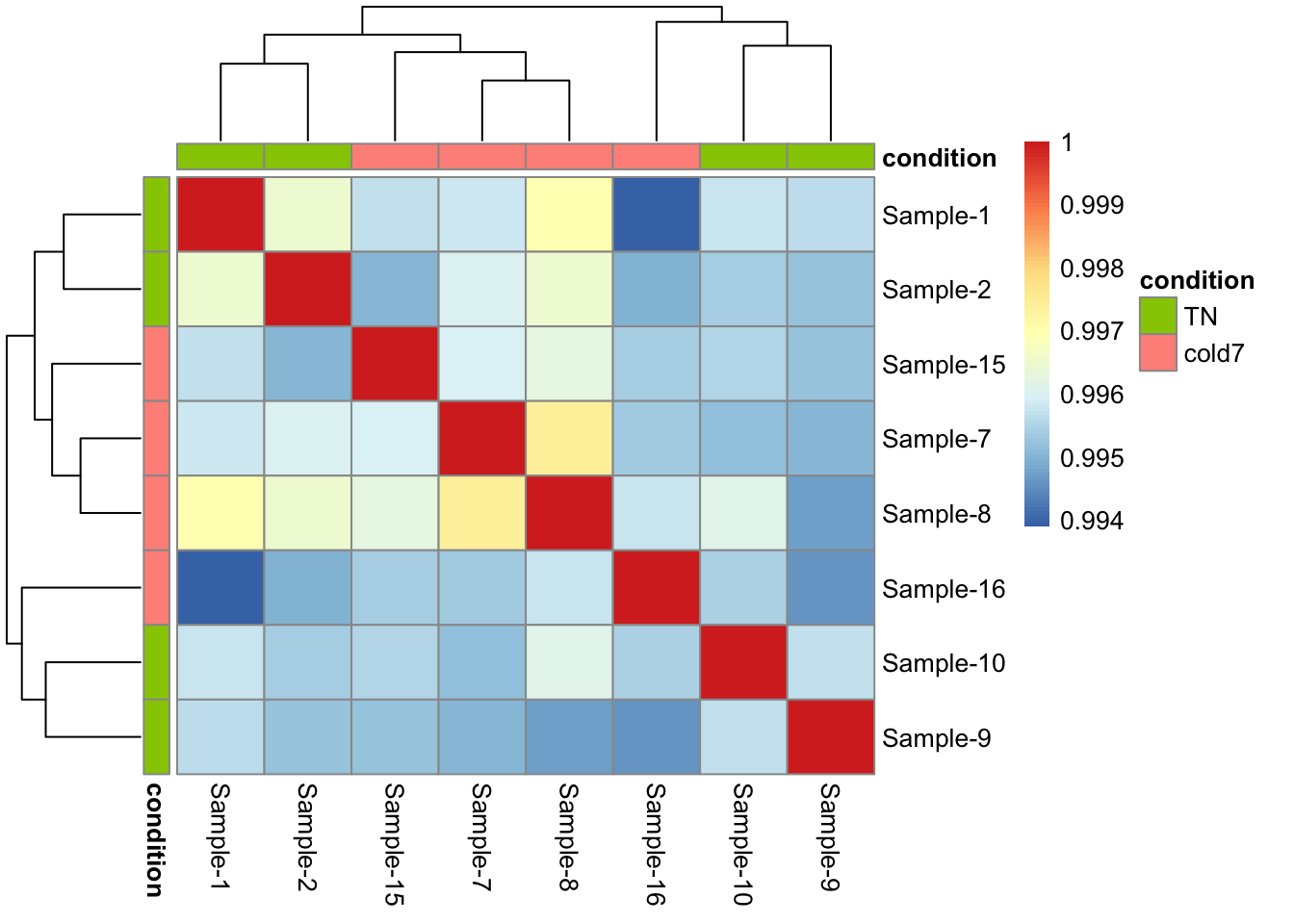

Unfortunately, the samples do not neatly separate by condition in this celltype. As shown in the PCA plot, three cold7 samples (7,8,15) are closely related on PC1, while the last cold7 sample (16) is more distant and groups with two TN samples (9,10) on PC2.

Exercise 2

Using the code below, run DESeq2 for the Pdgfr α+ APCs data. Following that draw the dispersion plot. Based on this plot do you think there is a reasonable fit to the model?

# Run DESeq2 differential expression analysis for APC
dds_APC <- DESeq(dds_APC)

# Run DESeq2 differential expression analysis
dds_APC <- DESeq(dds_APC)

# Plot gene-wise dispersion estimates to check model fit
plotDispEsts(dds_APC)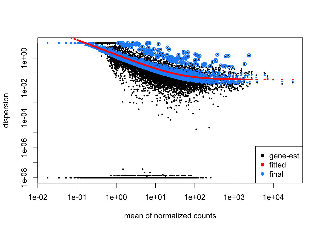

Exercise 3

Generate results for the Pdgfr α+ APCs and save it to a variable called res_APC. There is nothing to submit for this exercise, but please run the code as you will need res_APC for future exercises.

# Results of Wald test
res_APC <- results(dds_APC, 
                   contrast = contrast,
                   alpha = 0.05)

# Shrink the log2 fold changes to be more appropriate using the apeglm method
res_APC <- lfcShrink(dds_APC,
                     coef = "condition_cold7_vs_TN",
                     res  = res_APC,
                     type = "apeglm")