Set-up DESeq2 analysis - Answer Key

Exercise 1

Another cell type in this dataset that was particularly interesting to the authors were the Pdgfr α+ adipose progentior cells (APCs).

1. Subset the bulk object to isolate only adipose progenitor cells for the TN and cold7 conditions. Assign it to variable called bulk_APC.

Hint: You may need to review celltypes to determine what this cell type is called in our data. You can find unique celltypes with the code:

# Find unique celltypes
celltypes <- sort(unique(seurat@meta.data[["celltype"]]))

Note

The abbreviations for the cell types can be found in the project set-up lesson.

celltypes

[1] "Adipo"    "AP"       "EC"       "ECAP"     "Lymph"    "Pericyte" "Schwann" 
[8] "VSM"      "VSM-AP"  

# Compare TN vs cold7 in APC cells
bulk_APC <- subset(bulk, subset = (celltype == "AP")  & (condition %in% c("TN", "cold7")))

2. Plot the cell number distribution across samples. How do the numbers compare to VSM cells?

# Visualize number of cells per condition
ggplot(bulk_APC@meta.data, aes(x = sample, y = n_cells, fill = condition)) +
  geom_bar(stat = "identity", color = "black") +
  theme_classic() +
  theme(axis.text.x = element_text(angle = 45, vjust = 1, hjust = 1)) +
  labs(x = "Sample name", y = "Number of cells") +
  geom_text(aes(label = n_cells), vjust = -0.5)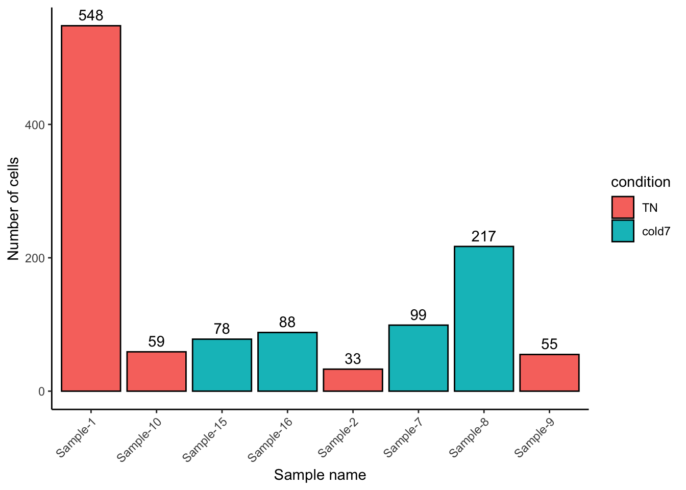

Click here for code to plot the two bar plots side-by-side

Note that this R code below uses the ggpubr library. In order to run this you will need to first install the package and then run:

library(ggpubr)

# Plot VSM and APC side by side
plot_cell_number_vsm <- ggplot(bulk_vsm@meta.data, aes(x = sample, y = n_cells, fill = condition)) +
  geom_bar(stat = "identity", color = "black") +
  theme_classic() +
  theme(axis.text.x = element_text(angle = 45, vjust = 1, hjust = 1)) +
  labs(x = "Sample name", y = "Number of cells") +
  geom_text(aes(label = n_cells), vjust = -0.5) +
  ggtitle("VSM") +
  theme(title = element_text(hjust = 0.5))

plot_cell_number_APC <- ggplot(bulk_APC@meta.data, aes(x = sample, y = n_cells, fill = condition)) +
  geom_bar(stat = "identity", color = "black") +
  theme_classic() +
  theme(axis.text.x = element_text(angle = 45, vjust = 1, hjust = 1)) +
  labs(x = "Sample name", y = "Number of cells") +
  geom_text(aes(label = n_cells), vjust = -0.5) +
  ggtitle("APC") +
  theme(title = element_text(hjust = 0.5))

ggpubr::ggarrange(plot_cell_number_vsm, plot_cell_number_APC, nrow = 1,
                  common.legend = TRUE, legend = "right")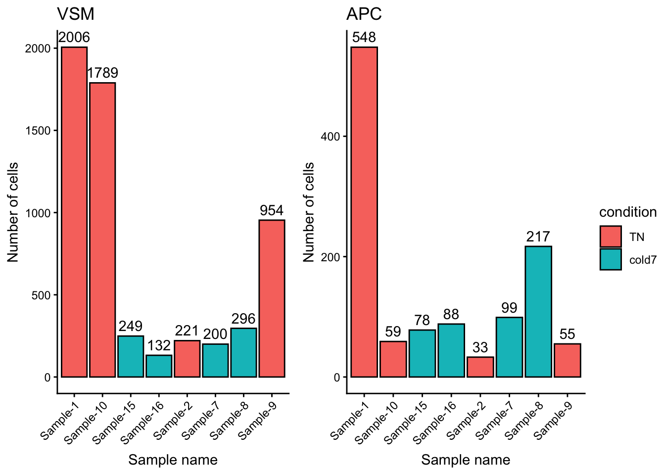

Overall we see far fewer cells, by an order of magnitude (scale goes to 2,000 for VSM but only 600 for APC). There is also a different distribution: the counts for Sample-10 and Sample-9 go down relative to other samples, while Sample-8 goes up.

Exercise 2

Create a DESeq2 object for the Pdgfr α+ APCs data as dds_APC.

# Get count matrix
APC_counts <- FetchData(bulk_APC, layer="counts", vars=rownames(bulk_APC))

# Create DESeq2 object
# transpose it to get genes as rows
dds_APC <- DESeqDataSetFromMatrix(t(APC_counts),
                                colData = bulk_APC@meta.data,
                                design = ~ condition)

dds_APC

class: DESeqDataSet 
dim: 19771 8 
metadata(1): version
assays(1): counts
rownames(19771): Xkr4 Gm1992 ... CAAA01118383.1 CAAA01147332.1
rowData names(0):
colnames(8): AP_Sample-1_TN AP_Sample-10_TN ... AP_Sample-8_cold7
  AP_Sample-9_TN
colData names(5): orig.ident celltype sample condition n_cells