Contributors: Meeta Mistry, Will Gammerdinger
Approximate time: 40 minutes
Learning Objectives
- Describe motifs and identify the general steps for a typical motif analysis
- Recognize tools for motif analysis
- Evaluate motif enrichment in H3K27Ac binding regions using the MEME suite
Motif analysis
After identifying regions of interest in the genome, there are various avenues to explore. In this workshop so far, we have demonstrated visualization of those regions using the read alignment data and we have annoated regions to identify nearest gene annotations and gained some biological context with functional analysis approaches. In this lesson, we discuss approaches for interrogating the actual sequence data corresponding to our regions/peaks of interest to evaluate enrichment of motif sequences.

Motifs are typically short, conserved sequences that have a specific biological significance, such as being binding sites for transcription factors (TFs), or other proteins that regulate gene expression. Motifs are often represented as Position-specific Weight Matrices (PWM), which is a matrix of 4 x m where m is the motif length. Every position in the matrix represents the probability of that nucleotide at each index position of the motif.
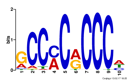
An example of the Klf4 motif from the JASPAR CORE database is displayed above.
Tools for motif analysis
There are a vast number of tools avaiable for motif finding. A 2014 study from Tran N.TL. and Huang C., reviewed nine web-based tools for detecting binding site motifs in ChIP-Seq data. Web-based tools are helpful as they provide a graphical user interface which makes it easy for the user to upload data and perform analysis. Many command-line tools also exist, as outlined in this benchmarking study in 2021 by Castellana S. et al. However, installation and the requirement of minimal technical skills can be identified as a limitation to some users.
Regardless of which tool you decide to use, the general steps involved will typically go as described below:
- Gather the sequences where there is supected presence of repeating motifs.
- The data set is scanned to look for sequences that appear frequently and are recurring in a way that is not just by random chance.
- Each potential pattern is evaluated based on how common it is and its significance value.
- Often the initial pattern search will result in many motifs, in which case some filtering is applied (too common, too rare, too similar to each other, etc.)
Once motifs have been discovered from the data, a common next step is to look for enrichment of known motifs by accessing public databases like JASPAR which is the largest open bioinformatics resource of TFBSs in the form of PWMs for eukaryotic genomes. Other commonly accessed resources include: HOCOMOCO which contains binding models for mouse and human transcription factors and TRANSFAC, a database of TFs, associated DNA motifs in eukaryotic genomes, and analysis tools.
The MEME Suite
In this workshop we will be using MEME (Multiple EM for Motif Elicitation) for motif discovery and motif enrichment. It is a web-based tool which has been shown to perform well in benchmarking studies using simulated data and in comparative studies with real ChIP-seq data. MEME is a tool which discovers novel, ungapped motifs (recurring, fixed-length patterns) in your sequences (sample output from sequences). MEME splits variable-length patterns into two or more separate motifs. STREME, is a very similar tool recommended for larger datasets (more than 50 sequences). Since we have many sequences, STREME is the better option for us.
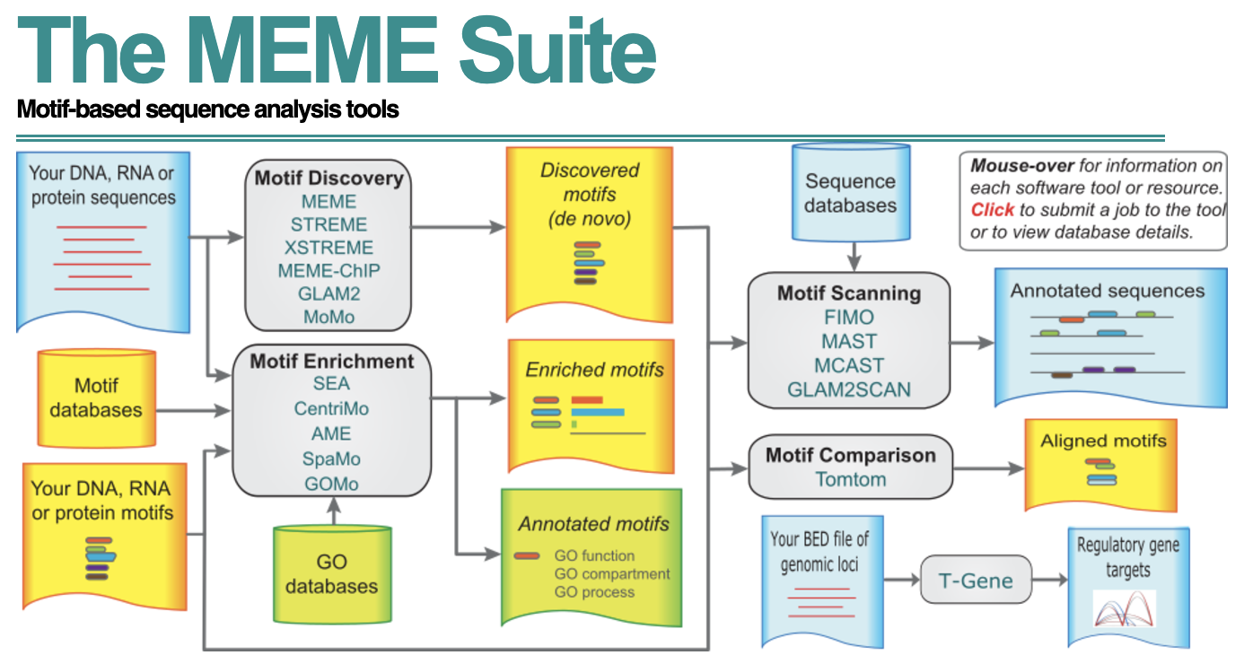
The web interface of MEME is easy to use, but there is also a stand-alone version if you prefer using it via the command-line tool. There is also a Bioconductor implementation, called the memes package, which provides a seamless R interface to a selection of popular MEME Suite tools. In addition to the analysis we perform in this workshop, there are various additional utility functions that we will not be covering but we encourage you to explore.
Prepare the data
STREME will accept BED files or sequence files as input, which must be in FASTA format. The data we will use as input will be a consensus set from the WT replicates. To generate the consensus set, we will access the olaps_wt variable created in a previous lesson. You should have this object in your environment.
Open up an R script file and call it motif_analysis_prep.R and add in a header line and the necessary libraries to load.
## Preparing data for motif analysis

# Load libraries
library(tidyverse)
library(GRanges)
library(ChIPseeker)
library(TxDb.Mmusculus. UCSC.mm10.knownGene)
Let’s begin by extracting the peaks which overlap across the replicates. Stored in the object are mergedPeaks, this corresponds to
an object of GRanges consisting of all merged overlapping peaks. Another option is peaksInMergedPeaks which is a GRanges object consisting of all peaks in each of the samples involved in the overlapping peaks. Since MEME/STREME suggests removing duplicate sequences, we will go with mergedPeaks. The only issue here is that merging might create some fairly large sized regions. MEME/STREME recommends the input sequence’s length should be ≤ 1,000 bp and as short as possible. As a result, we will filter the regions.
Click here if you are unable to locate olaps_wtcode in your environment
Run the code provided below to create the object
olaps_wt:
require(ChIPpeakAnno)
sample_files <- list.files(path = "./data/macs2/narrowPeak/", full.names = T)

# Reassign vars so that they are now GRanges instead of dataframes
for(r in 1:length(sample_files)){
  obj <- ChIPpeakAnno::toGRanges(sample_files[r], format="narrowPeak", header=FALSE)
  assign(vars[r], obj)
}

# Find overlapping peaks of WT samples
olaps_wt <- findOverlapsOfPeaks(WT_H3K27ac_ChIPseq_REP1,
                                WT_H3K27ac_ChIPseq_REP2,
                                WT_H3K27ac_ChIPseq_REP3, connectedPeaks = "merge")
# Get merged peaks for WT
wt_consensus <- olaps_wt$mergedPeaks

# Filter to keep only regions 1000bp or smaller
wt_consensus <- wt_consensus[width(wt_consensus) <= 1000]

# Remove non standard sequences as it will cause errors when retrieving the FASTA sequences from the reference (i.e. chr1_GL456211_random)
wt_consensus <- keepStandardChromosomes(wt_consensus, pruning.mode="coarse")
Since we are specifically interested in enhancer regions, we will annotate the consensus set and further filter this consensus set to only retain peaks that occur outside of promoter regions. We will create a minimal BED file with coordinates to use as input to STREME.
# Annotate consensus reiogns
annot_wt_consensus <- annotatePeak(wt_consensus, tssRegion = c(-3000, 3000),
                                   TxDb = TxDb.Mmusculus.UCSC.mm10.knownGene,
                                   annoDb = "org.Mm.eg.db")

# GRanges to dataframe
df <- annot_wt_consensus@anno %>% data.frame()

# Find regions annotated as "Promoter" and remove them
promoter_regions <- grep("Promoter", df$annotation)
non_promoter_df <- df[-(promoter_regions), ]

# Write minimal BED file
write_tsv(non_promoter_df[, 1:3], file = "results/non_promoter_wt.bed",
          col_names = F, quote = "none")
Running STREME
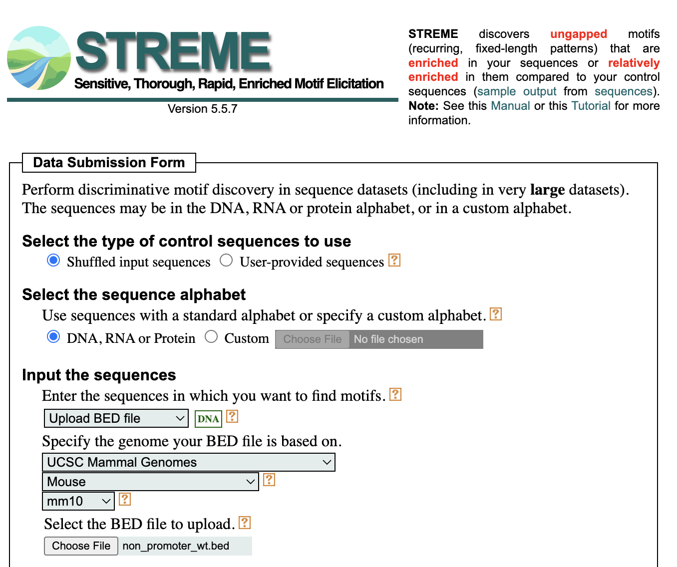
To run STREME, navigate to the MEME Suite web browser by clicking on this link. On the left hand side, locate the tools listed under “Motif Discovery”. Here, you will click on STREME, which will take you to the submission form depicted in the screenshot below. You will need to make the following selections:
- “Shuffled input sequences”
- STREME looks for motifs that are enriched in your sequences relative to a control set of sequences. This selection will create the control set by shuffling each of your input sequences, conserving k-mer frequencies, where k=3.
- The alternative is to provide a file of control sequences (be sure they have the same length distribution as the input)
- DNA, RNA or Protein sequence alphabet
- From the dropdown select Upload the BED file
- Select UCSC Mammal Genomes
- Select Mouse
- Select mm10
- Navigate and locate the
non_promoter_wt.bedfile we just created
- Enter your email if you would like email updates
Advanced options
If you click on Advanced Options you will see a host of selections we could make. They are described below, but note that we will be using default parameters.
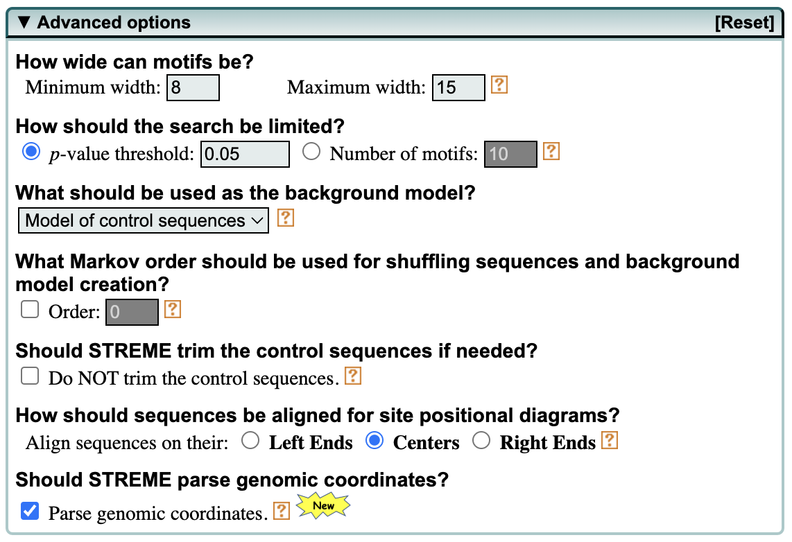
- The user can specify the minimum and maximum width for motifs.
- The number of sites for each motif can be provided, if there is prior knowledge about the number of occurrences that the motif has in the dataset.
- The p-value threshold can be modified to be more or less stringent.
- The background model normalizes for biased distribution of letters and groups of letters in your sequences. A 0-order model adjusts for single letter biases, a 1-order model adjusts for dimer biases (e.g., GC content in DNA sequences), etc. By default STREME uses m=2 for DNA and RNA sequences.
- Should the user choose to NOT trim the control sequences, this will cause STREME to use the (less accurate) Binomial test (instead of Fisher’s exact).
- Option to align sequences to the right or left. For visualizing motif distributions, center alignment is ideal for ChIP-seq and similar data.
STREME results
Once the tool is done running you will see a bullet point list of results generated, with each hyperlinked. The MEME suite tools provide three different output formats: HTML, XML and text. We will focus on the HTML report.
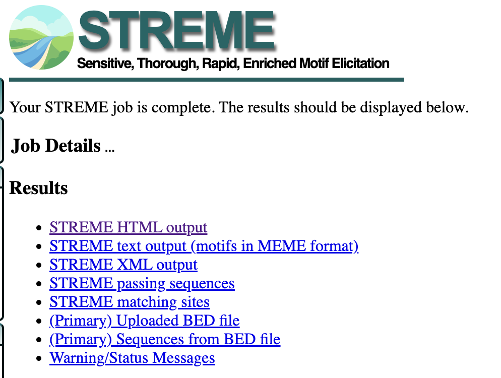
If you were not able to generate a result, click here to download the HTML report. For each motif, MEME outputs the p-value, E-value, the number of sites found, the motif’s logo (and reverse complement), and genomic coordinates for sites where the motifs were found. MEME also provides a Submit/Download option in HTML output for forwarding one or all motifs to other MEME programs for further analysis or downloading the the motif or logo.
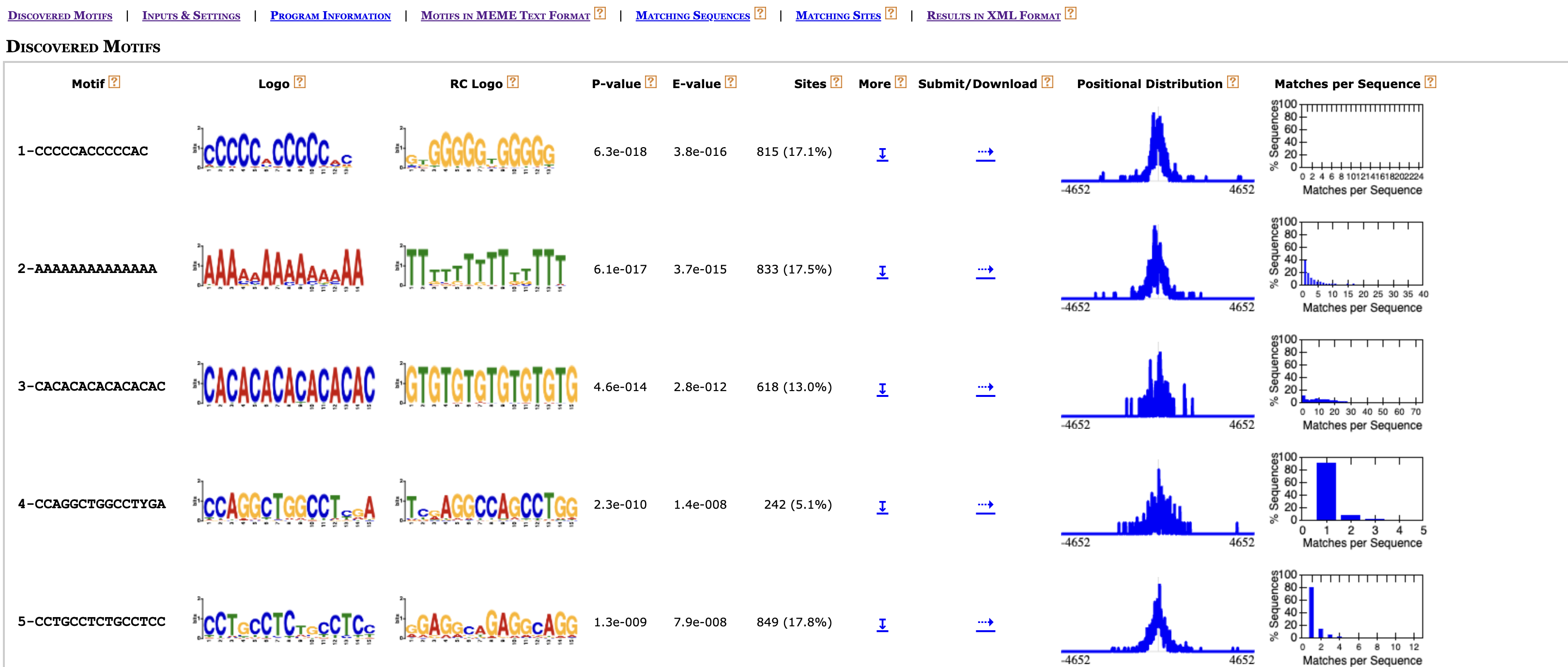
Let’s take a closer look at some of these results and see where we could explore further!
Consider the binding profile of H3K27Ac, where we observed a slight dip near the TSS in our profile plots. The motifs bound by transcription factors are most likely within the valleys of the H3K27ac signal. As such we might expect that some of the motifs from this report to align with binding motifs for transcriptional regulators, in particular those known to play a key role in cortical neurogenesis (since we are working wth cortical cells in mouse embryonic brain).
Scroll down in the report to motif 37-AGACAGATGG, and click on the Submit/Download button (can look like a sideways arrow). Here, choose the TomTom program to submit the motif.
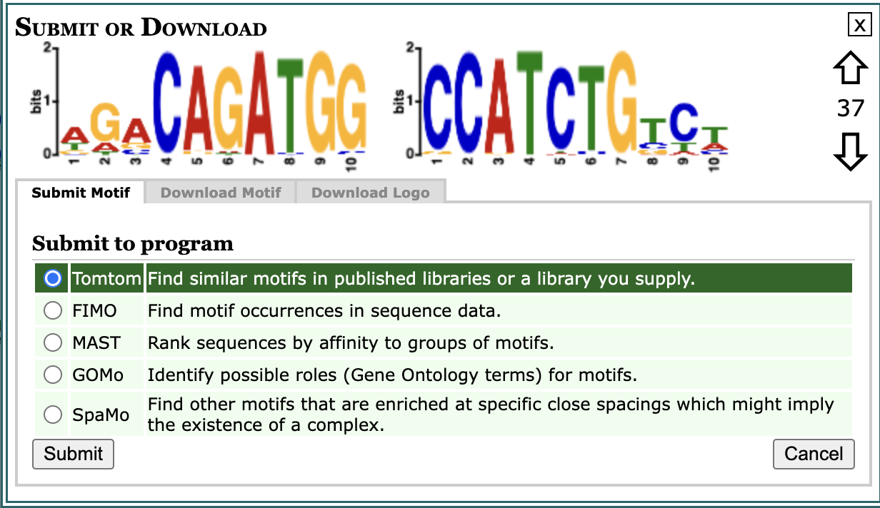
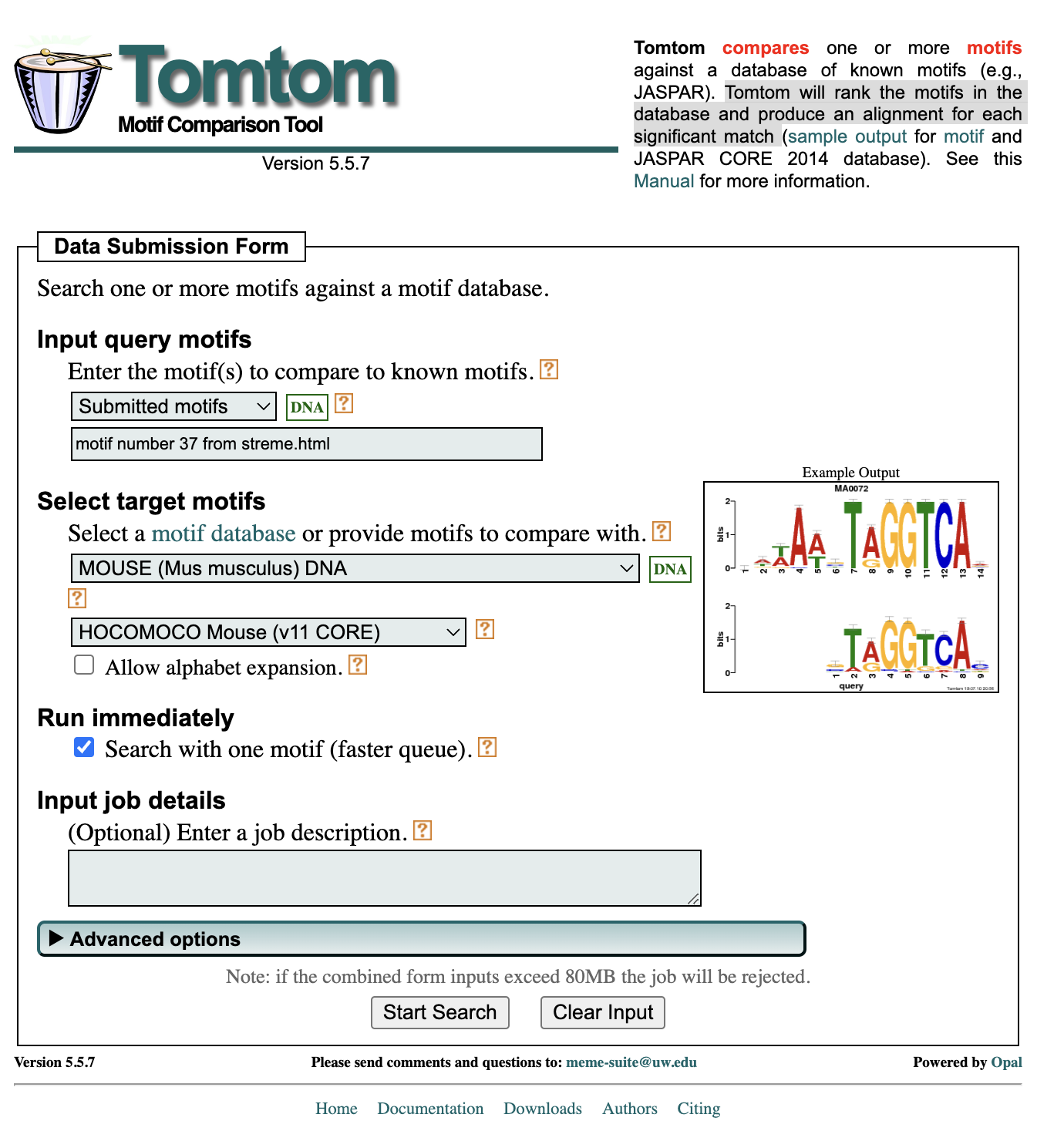
Once you hit submit you will find yourself at the data submission form for TomTom; a tool that compares a given motif against a database of known motifs. Tomtom will rank the motifs in the database and produce an alignment for each significant match.
- From the “Select target motifs” section you will choose MOUSE (Mus musculus) DNA.
- From the dropdown that appears below you will choose HOCOMOCO Mouse (v11 CORE).
- Then you can go ahead and “Start Search”.
After the result is generated, open up the HTML report in your browser. What you will find is that top hits for this motif sequence include NDF1, a transcriptional activator that associates with chromatin to enhancer regulatory elements in genes encoding key transcriptional regulators of neurogenesis. We also see ATOH1, a transcription factor which plays a role in the differentiation of subsets of neural cells and OLIG2 which regulates the differentiation of neural precursors into neurons, oligodendrocytes and astrocytes.
This is encouraging, as the result lines up with what we know about the regions used as input and the samples they originated from. While, we could continue to explore other motif results, another way of searching directly for known motifs would be to use a MEME program for Motif Enrichment (i.e. AME, or SEA).
Summary
In this lesson we have given you an introduction to motif analysis using an easy to navigate Web-tool called the MEME suite. This example demontrates the use of the tool for motif discovery, but also the utility of the MEME suite and other linked programs to continue to explore your data in more detail.
This lesson has been developed by members of the teaching team at the Harvard Chan Bioinformatics Core (HBC). These are open access materials distributed under the terms of the Creative Commons Attribution license (CC BY 4.0), which permits unrestricted use, distribution, and reproduction in any medium, provided the original author and source are credited.