Contributors: Mary Piper and Meeta Mistry
Approximate time: 1.25 hours
Learning Objectives
- Explore using lightweight algorithms to quantify reads to pseudocounts
- Understand how Salmon performs quasi-mapping and transcript abundance estimation
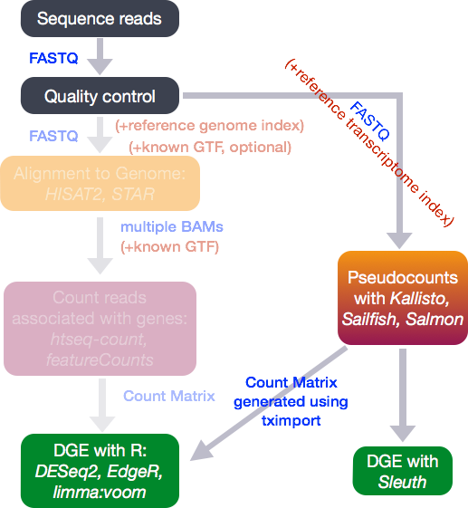
Lightweight alignment and quantification of gene expression
In the standard RNA-seq pipeline that we have presented so far, we have taken our reads post-QC and aligned them to the genome. The goal is to identify the genomic location where these reads originated from. Another strategy for quantification which has more recently been introduced involves transcriptome mapping. Tools that fall in this category include Kallisto, Sailfish and Salmon; each working slightly different from one another. (For this workshop we will explore Salmon in more detail.) Common to all of these tools is that base-to-base alignment of the reads is avoided, which is a time-consuming step, and these tools provide quantification estimates much faster than do standard approaches (typically more than 20 times faster) with improvements in accuracy at the transcript level. These transcript expression estimates, often referred to as ‘pseudocounts’, can be converted for use with DGE tools like DESeq2 or the estimates can be used directly for isoform-level differential expression using a tool like Sleuth.
The improvement in accuracy for lightweight alignment tools in comparison with the standard alignment/counting methods primarily relate to the ability of the lightweight alignment tools to quantify multimapping reads. This has been shown by Robert et. al by comparing the accuracy of 12 different alignment/quantification methods using simulated data to estimate the gene expression of 1000 perfect RNA-Seq read pairs from each of of the genes [1]. As shown in the figures below taken from the paper, the standard alignment and counting methods such as STAR/htseq or Tophat2/htseq result in underestimates of many genes - particularly those genes comprised of multimapping reads [1].
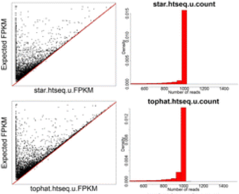
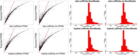
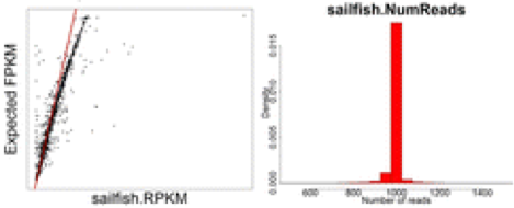
NOTE: Tails to the left indicate underestimates of gene expression, while tails to the right indicate overestimates of gene expression.
While the STAR/htseq standard method of alignment and counting is a bit conservative and can result in false negatives, Cufflinks tends to overestimate gene expression and results in many false positives, which is why Cufflinks is generally not recommended for gene expression quantification.
Finally, the most accurate quantification of gene expression was achieved using the lightweight alignment tool Sailfish (if used without bias correction).
Lightweight alignment tools such as Sailfish, Kallisto, and Salmon have generally been found to yield the most accurate estimations of transcript/gene expression. Salmon is considered to have some improvements relative to Sailfish, and it is considered to give very similar results to Kallisto.
What is Salmon?
Salmon is based on the philosophy of lightweight algorithms, which use the reference transcriptome (in FASTA format) and raw sequencing reads (in FASTQ format) as input, but do not align the full reads. These tools perform both mapping and quantification. Unlike most lightweight and standard alignment/quantification tools, Salmon utilizes sample-specific bias models for transcriptome-wide abundance estimation. Sample-specific bias models are helpful when needing to account for known biases present in RNA-Seq data including:
- GC bias
- positional coverage biases
- sequence biases at 5’ and 3’ ends of the fragments
- fragment length distribution
- strand-specific methods
If not accounted for, these biases can lead to unacceptable false positive rates in differential expression studies [2]. The Salmon algorithm can learn these sample-specific biases and account for them in the transcript abundance estimates. Salmon is extremely fast at “mapping” reads to the transcriptome and often more accurate than standard approaches [2].
How does Salmon estimate transcript abundances?
Similar to standard base-to-base alignment approaches, the quasi-mapping approach utilized by Salmon requires a reference index to determine the position and orientation information for where the fragments best map prior to quantification [3].
Indexing
This step involves creating an index to evaluate the sequences for all possible unique sequences of length k (kmer) in the transcriptome (genes/transcripts).
The index helps creates a signature for each transcript in our reference transcriptome. The Salmon index has two components:
- a suffix array (SA) of the reference transcriptome
- a hash table to map each transcript in the reference transcriptome to it’s location in the SA (is not required, but improves the speed of mapping drastically)
Quasi-mapping and quantification
The quasi-mapping approach estimates the numbers of reads mapping to each transcript, then generates final transcript abundance estimates after modeling sample-specific parameters and biases. The Rapmap tool [3] provides the underlying algorithm for the quasi-mapping.
NOTE: If there are sequences in the reads that are not in the index, they are not counted. As such, trimming is not required when using this method. Accordingly, if there are reads from transcripts not present in the reference transcriptome, they will not be quantified. Quantification of the reads is only as good as the quality of the reference transcriptome.
Running Salmon
First, start an interactive session, load the Salmon module and create a new directory for the Salmon results:
% srun --pty -p defq --qos=interactive --mem 8G bash

% module load Salmon
% mkdir ~/unix_lesson/rnaseq/salmon

% cd ~/unix_lesson/rnaseq/salmon
As you can imagine from the description above, when running Salmon there are also two steps.
Step 1: Indexing
“Index” the transcriptome using the index command:
## DO NOT RUN THIS CODE
% salmon index -t transcripts.fa -i transcripts_index --type quasi -k 31
NOTE: Default for salmon is –type quasi and -k 31, so we do not need to include these parameters in the index command. The kmer default of 31 is optimized for 75bp or longer reads, so if your reads are shorter, you may want a smaller kmer to use with shorter reads (kmer size needs to be an odd number).
We are not going to run this in class, but it only takes a few minutes. We will be using an index we have generated from transcript sequences (all known transcripts/ splice isoforms with multiples for some genes) for human. The transcriptome data (FASTA) was obtained from the Ensembl ftp site.
Step 2: Quantification:
Get the transcript abundance estimates using the quant command and the parameters described below (more information on parameters can be found here):
-i: specify the location of the index directory (/gstore/scratch/hpctrain/salmon.grch38_tx.idx/)-l: library type (single-end reverse readsSR, but we can useAto automatically infer the library type) - more information is available here)-r: list of files for sample (~/unix_lesson/rnaseq/raw_data/Mov10_oe_1.subset.fq)--useVBOpt: use variational Bayesian EM algorithm rather than the ‘standard EM’ to optimize abundance estimates (more accurate)-o: output quantification file name (Mov10_oe_1.subset.salmon)--writeMappings: instead of printing to screen, write to a file (--writeMappings=salmon.out)
To run the quantification step on a single sample we have the command provided below. Let’s try running it on our subset sample for Mov10_oe_1.subset.fq:
% salmon quant -i /gstore/scratch/hpctrain/salmon.grch38_tx.idx/ \
 -l SR \
 -r ~/unix_lesson/rnaseq/raw_data/Mov10_oe_1.subset.fq \
 -o Mov10_oe_1.subset.salmon \
 --writeMappings=salmon.out \
 --useVBOpt
NOTE: Paired-end reads require both sets of reads to be given in addition to a paired-end specific library type:
salmon quant -i transcripts_index -l <LIBTYPE> -1 reads1.fq -2 reads2.fq -o transcripts_quantTo have Salmon correct for RNA-Seq biases you will need to specify the appropriate parameters when you run it. Before using these parameters it is advisable to assess your data using tools like Qualimap to look specifically for the presence of these biases in your data and decide on which parameters would be appropriate.
To correct for the various sample-specific biases you could add the following parameters to the Salmon command:
--seqBiaswill enable it to learn and correct for sequence-specific biases in the input data.--gcBiasto learn and correct for fragment-level GC biases in the input data--posBiaswill enable modeling of a position-specific fragment start distribution
Salmon output
You should see a new directory has been created that is named by the string value you provided in the -o command. Take a look at what is contained in this directory:
% ls -l Mov10_oe_1.subset.salmon/
There is a logs directory, which contains all of the text that was printed to screen as Sailfish was running. Additionally, there is a file called quant.sf.
This is the quantification file in which each row corresponds to a transcript, listed by Ensembl ID, and the columns correspond to metrics for each transcript:
Name    Length  EffectiveLength TPM     NumReads
ENST00000632684.1       12      3.00168 0       0
ENST00000434970.2       9       2.81792 0       0
ENST00000448914.1       13      3.04008 0       0
ENST00000415118.1       8       2.72193 0       0
ENST00000631435.1       12      3.00168 0       0
ENST00000390567.1       20      3.18453 0       0
ENST00000439842.1       11      2.95387 0       0

....
- The first two columns are self-explanatory, the name of the transcript and the length of the transcript in base pairs (bp).
- The effective length represents the the various factors that effect the length of transcript due to technical limitations of the sequencing platform.
- Salmon outputs ‘pseudocounts’ which predict the relative abundance of different isoforms in the form of three possible metrics (KPKM, RPKM, and TPM). TPM (transcripts per million) is a commonly used normalization method as described in [1] and is computed based on the effective length of the transcript.
- Estimated number of reads (an estimate of the number of reads drawn from this transcript given the transcript’s relative abundance and length)
Running Salmon on multiple samples
We just ran Salmon on a single sample (and keep in mind a subset of chr1 from the original data). To obtain meaningful results we need to run this on all samples for the full dataset. To do so, we will create a shell script which will submit each Salmon run as a job to the cluster.
Open up a script in vim:
% vim salmon_all_samples.sh
Now we can create a for loop to iterate over all FASTQ samples, and submit a job to run Salmon on each sample in parallel. We begin by listing all BSUB directives to specify the resources we are requesting including memory, cores and wall time.
Next comes the Salmon command. Note, that we are adding a parameter called --numBootstraps to the Salmon command. Salmon has the ability to optionally compute bootstrapped abundance estimates. Bootstraps are required for estimation of technical variance. Bootstrapping essentially takes a different sub-sample of reads for each bootstapping run for estimating the transcript abundances. The technical variance is the variation in transcript abundance estimates calculated for each of the different sub-samplings (or bootstraps). We will discuss this in more detail in the next lesson.
NOTE: We are iterating over FASTQ files in the full dataset directory, located at
/gstore/scratch/hpctrain/full_dataset/
for fq in  /gstore/scratch/hpctrain/full_dataset/*fastq
 do
   base=$(basename $fq .fastq)
   sbatch -p defq --qos=short -c 6 --mem 8G \
   --wrap="salmon quant -i /gstore/scratch/hpctrain/salmon.grch38_tx.idx/ \
   -p 6 -l SR -r $fq --useVBOpt --numBootstraps 30 -o $base.salmon"
 done
Save and close the script. This is now ready to run. We are not going to run this script in class, since it might take a while.
NOTE: Window users will want to add the
--auxDirparameter to the Salmon command and provide an alternate name for the directory. By default it will be namedauxwhich interferes with the decompressing process when bringing files over locally to runtximport/DESeq2in R.
Next steps: Performing DE analysis on Pseudocounts
The pseudocounts generated by Salmon are represented as normalized TPM (transcripts per million) counts and map to transcripts or genes, depending on the input in the index step; in our case it was transcripts. These need to be converted into non-normalized count estimates for performing DE analysis using existing count-based tools.
Organizing the home directory
Since our home directory should contain only small scripts or files, we are going to move all workshop materials out of our home directory and into our scratch directory.
% cd

% echo $SCRATCH

% mv unix_lesson/rnaseq $SCRATCH
This lesson has been developed by members of the teaching team at the Harvard Chan Bioinformatics Core (HBC). These are open access materials distributed under the terms of the Creative Commons Attribution license (CC BY 4.0), which permits unrestricted use, distribution, and reproduction in any medium, provided the original author and source are credited.