Approximate time: 90 minutes
Learning Objectives:
- Describe and implement the RNA-seq workflow to align reads to the reference genome
- Describe tools and methods within the RNA-seq workflow
- Assessing input and output filetypes
Setting up to run the RNA-seq workflow
To get started with this lesson, we will start an interactive session and ask for 6 cores, by adding -c 6 to the srun command:
% srun --pty -p defq --qos=interactive -c 6 --mem 8G bash
Change directories into the rnaseq directory if not already there:
% cd ~/unix_lesson/rnaseq
You should have a directory tree setup similar to that shown below. It is best practice to have all files you intend on using for your workflow present within the same directory.
rnaseq/
	├── raw_data/
	├── meta/
	├── results/
	├── scripts/
	└── logs/
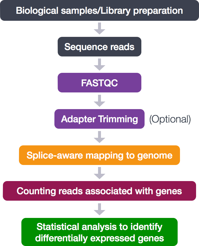
Below is a general overview of the steps involved in RNA-seq analysis.
So let’s get started by loading up some of the modules for tools we need for this section to perform alignment and assess the alignment:
% module load GMAP-GSNAP samtools
Create an output directory for our alignment files:
% mkdir results/gsnap
In the automation script, we will eventually loop over all of our files and have the cluster work on the files in parallel. For now, we’re going to work on just one to test and set up our workflow. To start we will use the first replicate in the Mov10 overexpression group, Mov10_oe_1_subset.fq.
Read Alignment
The alignment process consists of choosing an appropriate reference genome to map our reads against, and performing the read alignment using one of several splice-aware alignment tools such as GMAP-SNAP, STAR or HISAT2 (HISAT2 is a successor to both HISAT and TopHat2). The choice of aligner is a personal preference and also dependent on the computational resources that are available to you.
For this workshop we will be using GMAP-GSNAP, an aligner developed here at Genentech. This aligner is not just a splice-aware aligner for RNA-seq data, but it is versatile and is able to align various different types of DNA and protein inputs.
Originally developed over a decade ago, GMAP and GSNAP exhibit ongoing development to address continuing advancements in technology. The aligner utilizes different strategies for aligning reads, depending on the difficulty of alignment.
- Straightforward alignments: suffix arrays are used for the majority of easy-to-align reads resulting in efficient mapping.
- More difficult alignments: a hash table method is used for more difficult to align reads that the suffix arrays can miss.
- Reads not fully aligning with above methods: GSNAP has integrated the GMAP algorithm to take these partial alignments and use more computationally intensive methods to determine the most accurate alignments. GMAP was optimized to more accurately identify multiple indels and splice sites within a single read. For this reason, this tool is often recommended for long reads, such as those generated by Pacific Biosciences or MinION.
For more details regarding the GSNAP method please see the latest publication.
Running GMAP-GSNAP
Aligning reads using GMAP-GSNAP is a two-step process:
- Create a genome index
- Map reads to the genome
Creating a genome index
For this workshop we are using reads that originate from a small subsection of chromosome 1 (~300,000 reads) and so we are using only chr1 as the reference genome. Therefore, we cannot use any of the ready-made indices made available with the GMAP-SNAP install on the cluster (see note below for more information).
We have already created an index of chromosome1, which will be standing in for a reference genome. The indexing takes a lot longer than the actual alignment, and we can’t run it in class, but we have provided the code below that you would use to index the genome for your future reference.
** DO NOT RUN**
gmap_build -d <genome name> <path to genome fasta file>
Note: Contact the Bioinformatics & Computational Biology group for guidance if you want to modify the defaults for indexing.
Mapping RNA-seq reads
The inputs for mapping are the raw FASTQ files and the reference indices.
Basic options for mapping RNA-seq reads to the genome using GMAP-GSNAP:
-d: genome database (grch38_chr1)-D: genome directory (/gstore/scratch/hpctrain/chr1_reference_gsnap)-t: threads or cores (6)-M: report suboptimal hits beyond best hit (default=0) (2)-n: number of alignments that are maximally printed to the output per read (even if the read matches hundreds of times in the genome, which might happen with very short reads or reads spanning repetitive regions). (default = 100) (10)-N: look for novel splicing (default = 0 (no)) (1)
NOTE: If you are using the whole human genome, you would specify
-d GRCh38and there is no need to specify the path to the directory index, i.e. the-Doption.If you want to do the alignment against another genome, or a different version of the human genome contact the Bioinformatics & Computational Biology group for more information about which indices are available with the GMAP-GSNAP installation, and how to specify them with the
-doption.
Options we will keep as defaults, but including because it’s important not to change them for this workflow
--quality-protocol: quality encoding scale, with options including the old quality encoding (illumina) and the current quality encoding (sanger) (default = sanger)-w: definition of local novel splicing event (default = 200000 (i.e. local splicing events have the parts of reads within 200000 bases of each other))--pairmax-rna: max total genomic length for rna-seq paired reads or other reads that could have a splice (should likely match value for -w (default=200000)-E: distance splice penalty (where distant splice is an intron of length greater than value specified using -w OR is an inversion, scramble, or translocation between two different chromosomes) (default = 1)-A: output format type (options: sam, m8 (BLAST tabular format) (default = sam)-B: batch mode for using resources for fastest computation (default = 2)
Option important for paired-end reads, which will not affect single-end reads
--clip-overlap: for paired-end reads whose alignments overlap, clip overlapping region (won’t affect single-end reads)
Now let’s put it all together! The full GMAP-GSNAP alignment command is provided below.
If you like you can copy-paste it directly into your terminal. Alternatively, you can manually enter the command, but it is advisable to first type out the full command in a text editor (i.e. Sublime Text or Notepad++) on your local machine and then copy paste into the terminal. This will make it easier to catch typos and make appropriate changes.
% gsnap -d grch38_chr1 -D /gstore/scratch/hpctrain/chr1_reference_gsnap \
-t 6 -M 2 -n 10 -N 1 \
--quality-protocol=sanger -w 200000 --pairmax-rna=200000 \
-E 1 -B 2 \
-A sam raw_data/Mov10_oe_1.subset.fq | \
samtools view -bS - | \
samtools sort - \
 > results/gsnap/Mov10_oe_1.Aligned.sortedByCoord.out.bam
NOTE:
Other useful parameters:
- FASTQ files from the sequencer are often compressed, to align these files, GSNAP has the options
--gunzipand--bunzip2depending on the compression type.- Trimming the raw reads for poor quality and adapter sequences is not required as GSNAP performs soft-clipping by default. However, if you desire to perform your own trimming of mismatching sequences, you could turn off this feature using the parameter
--trim-mismatch-score=0.- If planning to perform other types of analyses, like intron retention analyses, bisulfite sequencing analysis, or chimeric analyses, among others, this versatile tool has specific parameters to change to optimize its use with these types of data.
Alignment Outputs (SAM/BAM)
The default output from GMAP-GSNAP is a SAM file, but we have used the pipe “|” to first convert it into a BAM file (see below), and then sort the entries (each read) in the BAM file by the genomic coordinates they align to.
When using the pipe with samtools, a special syntax is needed, wherein we need to use the hyphen “-“ after the command to let samtools know that the input for that command is being piped. You may encounter this with other tools as well.
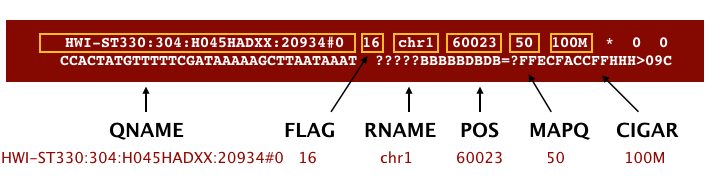
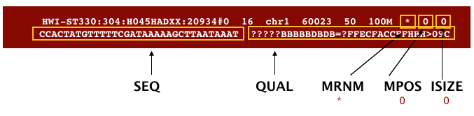
BAM is a binary version of the SAM file, also known as Sequence Alignment Map format. The SAM file is a tab-delimited text file that contains information for each individual read and its alignment to the genome. The file begins with an optional header (which starts with ‘@’), followed by an alignment section in which each line corresponds to alignment information for a single read. Each alignment line has 11 mandatory fields for essential mapping information and a variable number of fields for aligner specific information.
These fields are described briefly below, but for more detailed information the paper by Heng Li et al is a good start.
Let’s take a quick look at our alignment. To do so we first convert our BAM file into SAM format using samtools and then pipe it to the less command. This allows us to look at the contents without having to write it to file (since we don’t need a SAM file for downstream analyses).
% samtools view -h results/gsnap/Mov10_oe_1.Aligned.sortedByCoord.out.bam | less
Scroll through the SAM file and see how the fields correspond to what we expected.
Counting reads
Once we have our reads aligned to the genome, the next step is to count how many reads have been mapped to each gene. The input files required for counting include the BAM file and an associated gene annotation file in GTF format. htseq-count and featureCounts (part of the subread toolkit) are 2 commonly used counting tools. Today, we will be using featureCounts to get the gene counts. We picked this tool because it is accurate, fast and is relatively easy to use.
featureCounts works by taking the alignment coordinates for each read and cross-referencing that to the coordinates for features described in the GTF. Most commonly a feature is considered to be a gene, which is the union of all exons (which is also a feature type) that make up that gene. Please note that this tool is best used for counting reads associated with genes, and not for splice isoforms or transcripts, we will be covering that later today.
featureCounts only includes and counts those reads that map to a single location (uniquely mapping) and follows the scheme in the figure below for assigning reads to a gene/exon.
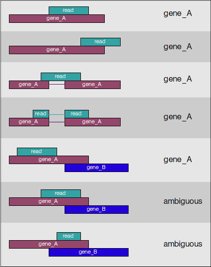
featureCounts can also take into account whether your data are stranded or not. If strandedness is specified, then in addition to considering the genomic coordinates it will also take the strand into account for counting. If your data are stranded always specify it.
Setting up to run featureCounts
Let’s start by creating a directory for the output and load the featureCounts module called subread:
% mkdir results/counts

% module load subread
How do we use this tool, what is the command and what options/parameters are available to us?
% featureCounts
So, it looks like the usage is featureCounts [options] -a <annotation_file> -o <output_file> input_file1 [input_file2] ... , where -a, -o and input files are required.
It can also take multiple bam files as input. Since we have only run GSNAP on 1 FASTQ file, let’s copy over the other bam files that we would need so we can generate the full count matrix.
% cp /gstore/scratch/hpctrain/bam_gsnap/*bam ~/unix_lesson/rnaseq/results/gsnap/
We are going to use the following options:
-T: number of threads or cores (6)-s: library strandedness with three possible values: 0 (unstranded), 1 (stranded) and 2 (reversely stranded (dUTP method)). 0 by default. For paired-end reads, strand of the first read is taken as the strand of the whole fragment. (2)
and the following are the values for the required parameters:
-a: path to GTF file (/gstore/scratch/hpctrain/chr1_reference_gsnap/chr1_grch38.gtf)-o: path to, and name of the output count matrix (~/unix_lesson/rnaseq/results/counts/Mov10_featurecounts.txt)- path to all of the bam files (
~/unix_lesson/rnaseq/results/gsnap/*bam)
Running featureCounts
% featureCounts -T 6 -s 2 \
  -a /gstore/scratch/hpctrain/chr1_reference_gsnap/chr1_grch38.gtf \
  -o ~/unix_lesson/rnaseq/results/counts/Mov10_featurecounts.txt \
  ~/unix_lesson/rnaseq/results/gsnap/*bam
featureCounts output
The output of this tool is 2 files, a count matrix and a summary file that tabulates how many the reads were “assigned” or counted and the reason they remained “unassigned”. Let’s take a look at the summary file:
% less results/counts/Mov10_featurecounts.txt.summary
Now let’s look at the count matrix:
% less results/counts/Mov10_featurecounts.txt
The count matrix that we need to perform differential gene expression analysis needs to look something like this:
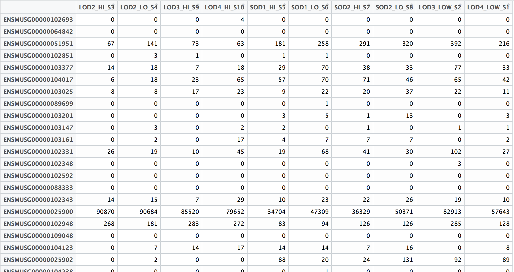
Since the featureCounts output has additional columns with information about genomic coordinates, gene length etc., we can use the cut command to select only those columns that you are interested in.
% cut -f1,7,8,9,10,11,12 results/counts/Mov10_featurecounts.txt > results/counts/Mov10_featurecounts.Rmatrix.txt
% less results/counts/Mov10_featurecounts.Rmatrix.txt
To ready this text file (count matrix) for the next step of differential gene expression analysis, you will need to clean it up further by removing the first header line, and modifying the column names (headers) to simpler, smaller sampleIDs. We can do this using a GUI text editor on our local laptops, or we can try using some of the shortcuts available in vim!
% vim results/counts/Mov10_featurecounts.Rmatrix.txt
Vim has nice shortcuts for cleaning up the header of our file using the following steps:
- Move the cursor to the beginning of the document by typing:
gg(in command mode). - Remove the first line by typing:
dd(in command mode). - Remove the file name following the sample name by typing:
:%s/_Aligned.sortedByCoord.out.bam//g(in command mode). - Remove the path leading up to the file name by typing:
:%s/\/gstore\/home\/username\/unix_lesson\/rnaseq\/results\/gsnap\///g(in command mode).
Note that we have a
\preceding each/, which tells vim that we are not using the/as part of our search and replace command, but instead the/is part of the pattern that we are replacing. This is called escaping the/.
Note on counting PE data
For paired-end (PE) data, the bam file contains information about whether both read1 and read2 mapped and if they were at roughly the correct distance from each other, that is to say if they were “properly” paired. For most counting tools, only properly paired reads are considered by default, and each read pair is counted only once as a single “fragment”.
For counting PE fragments associated with genes, the input bam files need to be sorted by read name (i.e. alignment information about both read pairs in adjoining rows). The alignment tool might sort them for you, but watch out for how the sorting was done. If they are sorted by coordinates (like with GSNAP), you will need to use
samtools sortto re-sort them by read name before using as input in featureCounts. If you do not sort you BAM file by read name before using as input, featureCounts assumes that almost all the reads are not properly paired.
Next Steps: Performing DE analysis on the count matrix
This text file with a matrix of raw counts can be used as input to tools like DESeq2, EdgeR and limma-voom. Running the DE analysis tools are outside the scope of this workshop since they require a working knowledge of R.
Visual assessment of the alignment
Index the BAM file for visualization with IGV:
% samtools index results/gsnap/Mov10_oe_1_Aligned.sortedByCoord.out.bam
Once we have the .bai index file to go with the .bam file, we can copy them over to our directory in the designated location to visualize with IGV.
% cp results/gsnap/Mov10_oe_1_Aligned.sortedByCoord.out.ba* /gne/web/dev/apache/htdocs/training/$USER
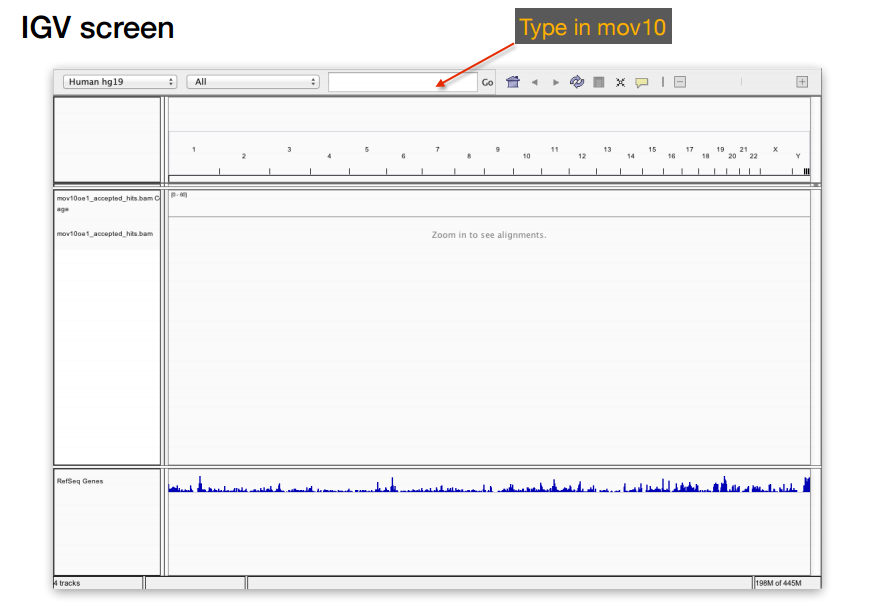
Visualize
- Start IGV, you should have this previously installed on your laptop.
- Load the Human genome (hg38) into IGV using the dropdown menu at the top left of your screen. If you can’t find hg38 right away, click on the “more..” at the bottom of the pull down menu and search for it using the search bar at the top.
Note: there is also an option to “Load Genomes from File…” under the “Genomes” pull-down menu - this is useful when working with non-model organisms or with fasta files that are unavailable in IGV.
- Use the “Load from URL…” option under the “File” pull-down menu and a box will pop up that will let you enter 2 URLs, one for the
.bamfiles and another for the.baifile (optional). Add the following URLs links in the appropriate input box:
http://resdev.gene.com/training/<your_username>/Mov10_oe_1_Aligned.sortedByCoord.out.bam
http://resdev.gene.com/training/<your_username>/Mov10_oe_1_Aligned.sortedByCoord.out.bam.bai
If not explicitly specified, IGV requires the
.baifile to be in the same location as corresponding.bamfile that you want to load into IGV, but there is no other direct use for this index file.*
Exercise
Now that we have done this for one sample, let’s try using the same commands to create a samtools index for the Irrel_kd_1_Aligned.sortedByCoord.out.bam file, and take the necessary steps to load it into IGV for visualization.
- How does the MOV10 gene look in the control sample in comparison to the overexpression sample?
- Take a look at a few other genes by typing into the search bar. For example, PPM1J and PTPN22. How do these genes compare?
- Thought question: Is loading
.bamfiles into IGV a valid way to compare expression between samples?
This lesson has been developed by members of the teaching team at the Harvard Chan Bioinformatics Core (HBC). These are open access materials distributed under the terms of the Creative Commons Attribution license (CC BY 4.0), which permits unrestricted use, distribution, and reproduction in any medium, provided the original author and source are credited.