Approximate time: 1.25 hours
Learning Objectives
- Explore using lightweight algorithms to quantify reads to pseudocounts
- Understand how Salmon performs quasi-mapping and transcript abundance estimation
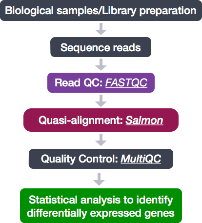
Lightweight alignment and quantification of gene expression
In the standard RNA-seq pipeline that we have presented so far, we have taken our reads post-QC and aligned them to the genome using our transcriptome annotation (GTF) as guidance. The goal is to identify the genomic location where these reads originated from. Another strategy for quantification which has more recently been introduced involves transcriptome mapping. Tools that fall in this category include Kallisto, Sailfish and Salmon; each working slightly different from one another. (For this workshop we will explore Salmon in more detail.) Common to all of these tools is that base-to-base alignment of the reads is avoided, which is a time-consuming step, and these tools provide quantification estimates much faster than do standard approaches (typically more than 20 times faster) with improvements in accuracy at the transcript level.
These transcript expression estimates, often referred to as ‘pseudocounts’, can be converted for use with DGE tools like DESeq2 (using tximport) or the estimates can be used directly for isoform-level differential expression using a tool like Sleuth.
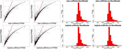
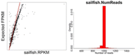
The improvement in accuracy for lightweight alignment tools in comparison with the standard alignment/counting methods primarily relate to the ability of the lightweight alignment tools to quantify multimapping reads. This has been shown by Robert et. al by comparing the accuracy of 12 different alignment/quantification methods using simulated data to estimate the gene expression of 1000 perfect RNA-Seq read pairs from each of of the genes [1]. As shown in the figures below taken from the paper, the standard alignment and counting methods such as STAR/htseq or Tophat2/htseq result in underestimates of many genes - particularly those genes comprised of multimapping reads [1].
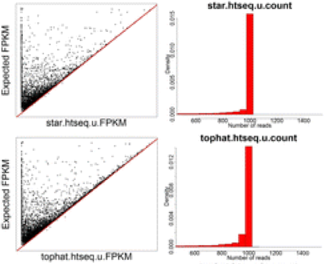
NOTE: Scatter plots are comparing FPKM for each of the 12 methods against the known FPKM from simulated data. The red line indicates the y = x line. For histograms of read counts, we expect a single peak at 1000 therefore tails represent over and under estimates.
While the STAR/htseq standard method of alignment and counting is a bit conservative and can result in false negatives, Cufflinks tends to overestimate gene expression and results in many false positives, which is why Cufflinks is generally not recommended for gene expression quantification.
Finally, the most accurate quantification of gene expression was achieved using the lightweight alignment tool Sailfish (if used without bias correction).
Lightweight alignment tools such as Sailfish, Kallisto, and Salmon have generally been found to yield the most accurate estimations of transcript/gene expression. Salmon is considered to have some improvements relative to Sailfish, and it is considered to give very similar results to Kallisto.
What is Salmon?
Salmon is based on the philosophy of lightweight algorithms, which use the reference transcriptome (in FASTA format) and raw sequencing reads (in FASTQ format) as input, but do not align the full reads. These tools perform both mapping and quantification. Unlike most lightweight and standard alignment/quantification tools, Salmon utilizes sample-specific bias models for transcriptome-wide abundance estimation. Sample-specific bias models are helpful when needing to account for known biases present in RNA-Seq data including:
- GC bias
- positional coverage biases
- sequence biases at 5’ and 3’ ends of the fragments
- fragment length distribution
- strand-specific methods
If not accounted for, these biases can lead to unacceptable false positive rates in differential expression studies [2]. The Salmon algorithm can learn these sample-specific biases and account for them in the transcript abundance estimates. Salmon is extremely fast at “mapping” reads to the transcriptome and often more accurate than standard approaches [2].
How does Salmon estimate transcript abundances?
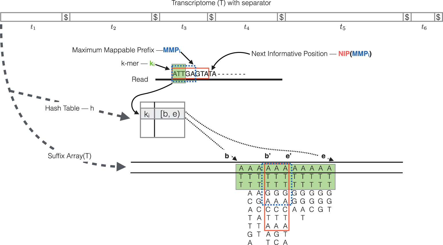
Similar to standard base-to-base alignment approaches, the quasi-mapping approach utilized by Salmon requires a reference index to determine the position and orientation information for where the fragments best map prior to quantification [3].
Indexing
This step involves creating an index to evaluate the sequences for all possible unique sequences of length k (kmer) in the transcriptome (genes/transcripts).
The index helps creates a signature for each transcript in our reference transcriptome. The Salmon index has two components:
- a suffix array (SA) of the reference transcriptome sequence
- a hash table to map each k-mer occurring in the reference transcriptome to it’s location in the SA (is not required, but improves the speed of mapping drastically)
Quasi-mapping and quantification
The quasi-mapping approach estimates the numbers of reads mapping to each transcript, and is described below. We have details and a schematic provided by the Rapmap tool [3], which provides the underlying algorithm for the quasi-mapping.
-
Step 1: Quasi mapping and abundance estimation
RapMap: a rapid, sensitive and accurate tool for mapping RNA-seq reads to transcriptomes. A. Srivastava, H. Sarkar, N. Gupta, R. Patro. Bioinformatics (2016) 32 (12): i192-i200.
The quasi-mapping procedure performs the following steps [3]:
- The read is scanned from left to right until a k-mer that appears in the hash table is discovered.
- The k-mer is looked up in the hash table and the SA intervals are retrieved, giving all suffixes containing that k-mer
- Similar to STAR, the maximal matching prefix (MMP) is identified by finding the longest read sequence that exactly matches the reference suffixes.
- Instead of searching for the next MMP in the read as we do with STAR, Salmon uses a k-mer skipping approach to identify the next informative position (NIP). In this way the SA search is likely to return a different set of transcripts than those returned for the previous MMP. Often natural variation or a sequencing error in the read is the cause of the mismatch from the reference, so beginning the search at this position would likely return the same set of transcripts.
- This process is repeated until the end of the read.
- The final set of mappings is determined by a consensus mechanism. Specifically, the algorithm reports the intersection of transcripts appearing in all MMPs for that read. The transcripts, orientation and transcript location are output for each read.
NOTE: If there are k-mers in the reads that are not in the index, they are not counted. As such, trimming is not required when using this method. Accordingly, if there are reads from transcripts not present in the reference transcriptome, they will not be quantified. Quantification of the reads is only as good as the quality of the reference transcriptome.
- Step 2: Improving abundance estimates Using multiple complex modeling approaches, like Expectation Maximization (EM), Salmon can also correct the abundance estimates for any sample-specific biases/factors [4]. Generally, this step results in more accurate transcript abundance estimation.
Running Salmon on O2
First start an interactive session and create a new directory for our Salmon analysis:
$ srun --pty -p short -t 0-12:00 --mem 8G --reservation=HBC /bin/bash

$ mkdir ~/unix_lesson/rnaseq/salmon

$ cd ~/unix_lesson/rnaseq/salmon
Salmon is not available as a module on O2, but it is installed as part of the bcbio pipeline. Since we already have the appropriate path (
/n/app/bcbio/tools/bin/) in our$PATHvariable we can use it by simply typing insalmon.
As you can imagine from the description above, when running Salmon there are also two steps.
Step 1: Indexing
“Index” the transcriptome using the index command:
## DO NOT RUN THIS CODE
$ salmon index -t transcripts.fa -i transcripts_index --type quasi -k 31
NOTE: Default for salmon is –type quasi and -k 31, so we do not need to include these parameters in the index command. The kmer default of 31 is optimized for 75bp or longer reads, so if your reads are shorter, you may want a smaller kmer to use with shorter reads (kmer size needs to be an odd number).
We are not going to run this in class, but it only takes a few minutes. We will be using an index we have generated from transcript sequences (all known transcripts/ splice isoforms with multiples for some genes) for human. The transcriptome data (FASTA) was obtained from the Ensembl ftp site.
Step 2: Quantification:
Get the transcript abundance estimates using the quant command and the parameters described below (more information on parameters can be found here):
-i: specify the location of the index directory; for us it isn/groups/hbctraining/ngs-data-analysis-longcourse/rnaseq/salmon.ensembl38.idx-l A: auto-detect library type. You can also specify stranded single-end reads, more info available here-r: list of files for sample-o: output quantification file name--seqBiaswill enable Salmon to learn and correct for sequence-specific biases in the input data--useVBOpt: use variational Bayesian EM algorithm rather than the ‘standard EM’ to optimize abundance estimates (more accurate)--writeMappings=salmon.out: creates a SAM-like file of all of the mappings. We won’t add this parameter, as it creates large files that will take up too much space in your home directory.
To run the quantification step on a single sample we have the command provided below. Let’s try running it on our subset sample for Mov10_oe_1.subset.fq:
$ salmon quant -i /n/groups/hbctraining/ngs-data-analysis-longcourse/rnaseq/salmon.ensembl38.idx \
 -l A \
 -r ~/unix_lesson/rnaseq/raw_data/Mov10_oe_1.subset.fq \
 -o Mov10_oe_1.subset.salmon \
 --seqBias \
 --useVBOpt
NOTE 1: Paired-end reads require both sets of reads to be given in addition to a paired-end specific library type:
salmon quant -i transcripts_index -l <LIBTYPE> -1 reads1.fq -2 reads2.fq -o transcripts_quant
NOTE 2: To have Salmon correct for other RNA-Seq biases you will need to specify the appropriate parameters when you run it. Before using these parameters it is advisable to assess your data using tools like Qualimap to look specifically for the presence of these biases in your data and decide on which parameters would be appropriate.
To correct for the various sample-specific biases you could add the following parameters to the Salmon command:
--gcBiasto learn and correct for fragment-level GC biases in the input data--posBiaswill enable modeling of a position-specific fragment start distribution
Salmon output
You should see a new directory has been created that is named by the string value you provided in the -o command. Take a look at what is contained in this directory:
$ ls -l Mov10_oe_1.subset.salmon/
There is a logs directory, which contains all of the text that was printed to screen as Sailfish was running. Additionally, there is a file called quant.sf.
This is the quantification file in which each row corresponds to a transcript, listed by Ensembl ID, and the columns correspond to metrics for each transcript:
Name    Length  EffectiveLength TPM     NumReads
ENST00000456328 1657    1407.000        0.000000        0.000
ENST00000450305 632     382.000 0.000000        0.000
ENST00000488147 1351    1101.000        0.000000        0.000
ENST00000619216 68      3.000   0.000000        0.000
ENST00000473358 712     462.000 0.000000        0.000
ENST00000469289 535     285.000 0.000000        0.000
ENST00000607096 138     5.000   0.000000        0.000
ENST00000417324 1187    937.000 0.000000        0.000

....
- The first two columns are self-explanatory, the name of the transcript and the length of the transcript in base pairs (bp).
- The effective length represents the various factors that effect the length of transcript (i.e degradation, technical limitations of the sequencing platform)
- Salmon outputs ‘pseudocounts’ which predict the relative abundance of different isoforms in the form of three possible metrics (KPKM, RPKM, and TPM). TPM (transcripts per million) is a commonly used normalization method as described in [1] and is computed based on the effective length of the transcript.
- Estimated number of reads (an estimate of the number of reads drawn from this transcript given the transcript’s relative abundance and length)
Running Salmon on multiple samples
We just ran Salmon on a single sample (and keep in mind only on a subset of chr1 from the original data). To obtain meaningful results we need to run this on all samples for the full dataset. To do so, we will need to create a job submission script.
NOTE: We are iterating over FASTQ files in the full dataset directory, located at
/n/groups/hbctraining/ngs-data-analysis-longcourse/rnaseq/full_dataset
Create a job submission script to run Salmon in serial
Since Salmon is only able to take a single file as input, one way in which we can do this is to use a for loop to run Salmon on all samples in serial. What this means is that Salmon will process the dataset one sample at a time.
Let’s start by opening up a script in vim:
$ vim salmon_all_samples.sbatch
Let’s start our script with a shebang line followed by SBATCH directives which describe the resources we are requesting from O2. We will ask for 6 cores and take advantage of Salmon’s multi-threading capabilities. Note that we also removed the --reservation from our SBATCH options.
Next we will do the following:
- Create a for loop to iterate over all FASTQ samples.
- Inside the loop we will create a variable that stores the prefix we will use for naming output files.
- Then we run Salmon.
NOTE: We have added a couple of new parameters. First, since we are multithreading with 6 cores we will use
-p 6. Another new parameter we have added is called--numBootstraps. Salmon has the ability to optionally compute bootstrapped abundance estimates. Bootstraps are required for estimation of technical variance. We will discuss this in more detail when we talk about transcript-level differential expression analysis.
The final script is shown below:
#!/bin/bash

#SBATCH -p short
#SBATCH -c 6
#SBATCH -t 0-12:00
#SBATCH --mem 8G
#SBATCH --job-name salmon_in_serial
#SBATCH -o %j.out
#SBATCH -e %j.err

cd ~/unix_lesson/rnaseq/salmon

for fq in /n/groups/hbctraining/ngs-data-analysis-longcourse/rnaseq/full_dataset/*.fastq

do

# create a prefix
base=`basename $fq .fastq`

# run salmon
salmon quant -i /n/groups/hbctraining/ngs-data-analysis-longcourse/rnaseq/salmon.ensembl38.idx \
 -l A \
 -r $fq \
 -p 6 \
 -o $base.salmon \
 --seqBias \
 --useVBOpt \
 --numBootstraps 30

done
Save and close the script. This is now ready to run.
$ sbatch salmon_all_samples.sbatch
Once you have run Salmon on all of your samples, you will need to decide whether you would like to perform gene-level or isoform-level analysis. The output directory from Salmon for each sample will be required as input for any of these downstream tools. In our standard workflow we ended up with a count matrix where all expression data was nicely summarized into a single file, but with this alternative approach the downstream tools for differential expression will take care of compiling it for you.
Exercise
We learned in the Automation lesson that we can be more efficient by running our jobs in parallel. In this way, each sample is run as an independent job and not waiting for the previous sample to finish. Create a new script to run Salmon in parallel.
This lesson has been developed by members of the teaching team at the Harvard Chan Bioinformatics Core (HBC). These are open access materials distributed under the terms of the Creative Commons Attribution license (CC BY 4.0), which permits unrestricted use, distribution, and reproduction in any medium, provided the original author and source are credited.