Data subsetting with base R: vectors and factors

Approximate time: 60 min

Learning Objectives

Construct data structures to store external data in R.
Inspect data structures in R.
Demonstrate how to subset data from data structures.

Reading data into R

Regardless of the specific analysis in R we are performing, we usually need to bring data in for the analysis. The function in R we use will depend on the type of data file we are bringing in (e.g. text, Stata, SPSS, SAS, Excel, etc.) and how the data in that file are separated, or delimited. The table below lists functions that can be used to import data from common file formats.

Data type	Extension	Function	Package
Comma separated values	csv	`read.csv()`	utils (default)
		`read_csv()`	readr (tidyverse)
Tab separated values	tsv	`read_tsv()`	readr
Other delimited formats	txt	`read.table()`	utils
		`read_table()`	readr
		`read_delim()`	readr
Stata version 13-14	dta	`readdta()`	haven
Stata version 7-12	dta	`read.dta()`	foreign
SPSS	sav	`read.spss()`	foreign
SAS	sas7bdat	`read.sas7bdat()`	sas7bdat
Excel	xlsx, xls	`read_excel()`	readxl (tidyverse)

For example, if we have text file separated by commas (comma-separated values), we could use the function read.csv. However, if the data are separated by a different delimiter in a text file, we could use the generic read.table function and specify the delimiter as an argument in the function.

When working with genomic data, we often have a metadata file containing information on each sample in our dataset. Let’s bring in the metadata file using the read.csv function. Check the arguments for the function to get an idea of the function options:

?read.csv

The read.csv function has one required argument and several options that can be specified. The mandatory argument is a path to the file and filename, which in our case is data/mouse_exp_design.csv. We will put the function to the right of the assignment operator, meaning that any output will be saved as the variable name provided on the left.

metadata <- read.csv(file="data/mouse_exp_design.csv")

Note: By default, read.csv converts (= coerces) columns that contain characters (i.e., text) into the factor data type. Depending on what you want to do with the data, you may want to keep these columns as character. To do so, read.csv() and read.table() have an argument called stringsAsFactors which can be set to FALSE.

Inspecting data structures

There are a wide selection of base functions in R that are useful for inspecting your data and summarizing it. Let’s use the metadata file that we created to test out data inspection functions.

Take a look at the dataframe by typing out the variable name metadata and pressing return; the variable contains information describing the samples in our study. Each row holds information for a single sample, and the columns contain categorical information about the sample genotype(WT or KO), celltype (typeA or typeB), and replicate number (1,2, or 3).

metadata

          genotype celltype replicate
sample1        Wt    typeA		1
sample2        Wt    typeA		2
sample3        Wt    typeA		3
sample4        KO    typeA		1
sample5        KO    typeA		2
sample6        KO    typeA		3
sample7        Wt    typeB		1
sample8        Wt    typeB		2
sample9        Wt    typeB		3
sample10       KO    typeB		1
sample11       KO    typeB		2
sample12       KO    typeB		3

Suppose we had a larger file, we might not want to display all the contents in the console. Instead we could check the top (the first 6 lines) of this data.frame using the function head():

head(metadata)

Previously, we had mentioned that character values get converted to factors by default using data.frame. One way to assess this change would be to use the __str__ucture function. You will get specific details on each column:

str(metadata)

'data.frame':	12 obs. of  3 variables:
 $ genotype : Factor w/ 2 levels "KO","Wt": 2 2 2 1 1 1 2 2 2 1 ...
 $ celltype : Factor w/ 2 levels "typeA","typeB": 1 1 1 1 1 1 2 2 2 2 ...
 $ replicate: num  1 2 3 1 2 3 1 2 3 1 ...

As you can see, the columns genotype and celltype are of the factor class, whereas the replicate column has been interpreted as integer data type.

You can also get this information from the “Environment” tab in RStudio.

List of functions for data inspection

We already saw how the functions head() and str() can be useful to check the content and the structure of a data.frame. Here is a non-exhaustive list of functions to get a sense of the content/structure of data.

All data structures - content display:
- str(): compact display of data contents (env.)
- class(): data type (e.g. character, numeric, etc.) of vectors and data structure of dataframes, matrices, and lists.
- summary(): detailed display, including descriptive statistics, frequencies
- head(): will print the beginning entries for the variable
- tail(): will print the end entries for the variable
Vector and factor variables:
- length(): returns the number of elements in the vector or factor
Dataframe and matrix variables:
- dim(): returns dimensions of the dataset
- nrow(): returns the number of rows in the dataset
- ncol(): returns the number of columns in the dataset
- rownames(): returns the row names in the dataset
- colnames(): returns the column names in the dataset

Selecting data using indices and sequences

When analyzing data, we often want to partition the data so that we are only working with selected columns or rows. A data frame or data matrix is simply a collection of vectors combined together. So let’s begin with vectors and how to access different elements, and then extend those concepts to dataframes.

Vectors

Selecting using indices

If we want to extract one or several values from a vector, we must provide one or several indices using square brackets [ ] syntax. The index represents the element number within a vector (or the compartment number, if you think of the bucket analogy). R indices start at 1. Programming languages like Fortran, MATLAB, and R start counting at 1, because that’s what human beings typically do. Languages in the C family (including C++, Java, Perl, and Python) count from 0 because that’s simpler for computers to do.

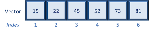
Let’s start by creating a vector called age:

age <- c(15, 22, 45, 52, 73, 81)

vector indices

Suppose we only wanted the fifth value of this vector, we would use the following syntax:

age[5]

If we wanted all values except the fifth value of this vector, we would use the following:

age[-5]

If we wanted to select more than one element we would still use the square bracket syntax, but rather than using a single value we would pass in a vector of several index values:

age[c(3,5,6)]   ## nested

# OR

## create a vector first then select
idx <- c(3,5,6) # create vector of the elements of interest
age[idx]

To select a sequence of continuous values from a vector, we would use : which is a special function that creates numeric vectors of integer in increasing or decreasing order. Let’s select the first four values from age:

age[1:4]

Alternatively, if you wanted the reverse could try 4:1 for instance, and see what is returned.

Exercises

Create a vector called alphabets with the following letters, C, D, X, L, F.
Use the associated indices along with [ ] to do the following:
- only display C, D and F
- display all except X
- display the letters in the opposite order (F, L, X, D, C)

Selecting using indices with logical operators

We can also use indices with logical operators. Logical operators include greater than (>), less than (<), and equal to (==). A full list of logical operators in R is displayed below:

Operator	Description
>	greater than
>=	greater than or equal to
<	less than
<=	less than or equal to
==	equal to
!=	not equal to
&	and
\|	or

We can use logical expressions to determine whether a particular condition is true or false. For example, let’s use our age vector:

age

If we wanted to know if each element in our age vector is greater than 50, we could write the following expression:

age > 50

Returned is a vector of logical values the same length as age with TRUE and FALSE values indicating whether each element in the vector is greater than 50.

[1] FALSE FALSE FALSE  TRUE  TRUE  TRUE

We can use these logical vectors to select only the elements in a vector with TRUE values at the same position or index as in the logical vector.

Select all values in the age vector over 50 or age less than 18:

age > 50 | age < 18

age

age[age > 50 | age < 18]  ## nested

# OR

## create a vector first then select
idx <- age > 50 | age < 18
age[idx]

Indexing with logical operators using the `which()` function

While logical expressions will return a vector of TRUE and FALSE values of the same length, we could use the which() function to output the indices where the values are TRUE. Indexing with either method generates the same results, and personal preference determines which method you choose to use. For example:

which(age > 50 | age < 18)

age[which(age > 50 | age < 18)]  ## nested

# OR

## create a vector first then select
idx_num <- which(age > 50 | age < 18)
age[idx_num]

Notice that we get the same results regardless of whether or not we use the which(). Also note that while which() works the same as the logical expressions for indexing, it can be used for multiple other operations, where it is not interchangeable with logical expressions.

Factors

Since factors are special vectors, the same rules for selecting values using indices apply. The elements of the expression factor created previously had the following categories or levels: low, medium, and high.

Let’s extract the values of the factor with high expression, and let’s using nesting here:

expression[expression == "high"]    ## This will only return those elements in the factor equal to "high"

Nesting note:

The piece of code above was more efficient with nesting; we used a single step instead of two steps as shown below:

Step1 (no nesting): idx <- expression == "high"

Step2 (no nesting): expression[idx]

Exercise

Extract only those elements in samplegroup that are not KO (nesting the logical operation is optional).

Releveling factors

We have briefly talked about factors, but this data type only becomes more intuitive once you’ve had a chance to work with it. Let’s take a slight detour and learn about how to relevel categories within a factor.

To view the integer assignments under the hood you can use str():

expression

str(expression)
Factor w/ 3 levels "high","low","medium": 2 1 3 1 2 3 1

The categories are referred to as “factor levels”. As we learned earlier, the levels in the expression factor were assigned integers alphabetically, with high=1, low=2, medium=3. However, it makes more sense for us if low=1, medium=2 and high=3, i.e. it makes sense for us to “relevel” the categories in this factor.

To relevel the categories, you can add the levels argument to the factor() function, and give it a vector with the categories listed in the required order:

expression <- factor(expression, levels=c("low", "medium", "high"))     # you can re-factor a factor 

str(expression)
Factor w/ 3 levels "low","medium",..: 1 3 2 3 1 2 3

Now we have a releveled factor with low as the lowest or first category, medium as the second and high as the third. This is reflected in the way they are listed in the output of str(), as well as in the numbering of which category is where in the factor.

Note: Releveling becomes necessary when you need a specific category in a factor to be the “base” category, i.e. category that is equal to 1. One example would be if you need the “control” to be the “base” in a given RNA-seq experiment.