Introduction to R - ARCHIVED

Approximate time: 45 minutes

Learning Objectives

• Describe what R and RStudio are.
• Interact with R using RStudio.
• Use the various components of RStudio.

What is R?

The common misconception is that R is a programming language but in fact it is much more than that. Think of R as an environment for statistical computing and graphics, which brings together a number of features to provide powerful functionality.

The R environment combines:

• effective handling of big data
• collection of integrated tools
• graphical facilities
• simple and effective programming language

Why use R?

R is a powerful, extensible environment. It has a wide range of statistics and general data analysis and visualization capabilities.

• Data handling, wrangling, and storage
• Wide array of statistical methods and graphical techniques available
• Easy to install on any platform and use (and it’s free!)
• Open source with a large and growing community of peers

What is RStudio?

RStudio is freely available open-source Integrated Development Environment (IDE). RStudio provides an environment with many features to make using R easier and is a great alternative to working on R in the terminal.

• Graphical user interface, not just a command prompt
• Great learning tool
• Free for academic use
• Platform agnostic
• Open source

Creating a new project directory in RStudio

Let’s create a new project directory for our “Introduction to R” lesson today.

1. Open RStudio
2. Go to the File menu and select New Project.
3. In the New Project window, choose New Directory. Then, choose New Project. Name your new directory Intro-to-R and then “Create the project as subdirectory of:” the Desktop (or location of your choice).
4. Click on Create Project.
5. After your project is completed, if the project does not automatically open in RStudio, then go to the File menu, select Open Project, and choose Intro-to-R.Rproj.
6. When RStudio opens, you will see three panels in the window.
7. Go to the File menu and select New File, and select R Script. The RStudio interface should now look like the screenshot below.

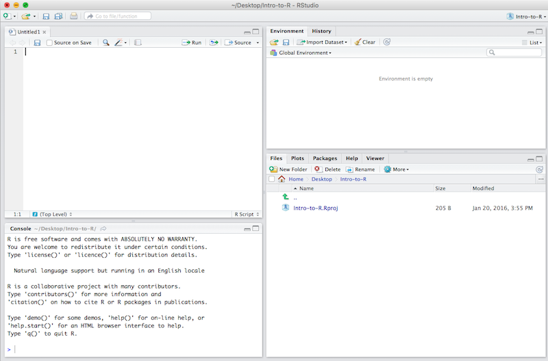
RStudio Interface

The RStudio interface has four main panels:

1. Console: where you can type commands and see output. The console is all you would see if you ran R in the command line without RStudio.
2. Script editor: where you can type out commands and save to file. You can also submit the commands to run in the console.
3. Environment/History: environment shows all active objects and history keeps track of all commands run in console
4. Files/Plots/Packages/Help

Organizing your working directory & setting up

Viewing your working directory

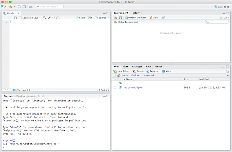
Before we organize our working directory, let’s check to see where our current working directory is located by typing into the console:

getwd()

Your working directory should be the Intro-to-R folder constructed when you created the project. The working directory is where RStudio will automatically look for any files you bring in and where it will automatically save any files you create, unless otherwise specified.

You can visualize your working directory by selecting the Files tab from the Files/Plots/Packages/Help window.

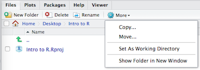
If you wanted to choose a different directory to be your working directory, you could navigate to a different folder in the Files tab, then, click on the More dropdown menu and select Set As Working Directory.

Structuring your working directory

To organize your working directory for a particular analysis, you should separate the original data (raw data) from intermediate datasets. For instance, you may want to create a data/ directory within your working directory that stores the raw data, and have a results/ directory for intermediate datasets and a figures/ directory for the plots you will generate.

Let’s create these three directories within your working directory by clicking on New Folder within the Files tab.

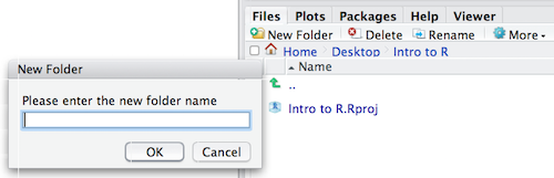
When finished, your working directory should look like:

Setting up

This is more of a housekeeping task. We will be writing long lines of code in our script editor and want to make sure that the lines “wrap” and you don’t have to scroll back and forth to look at your long line of code.

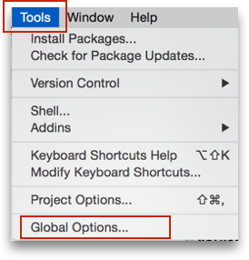
Click on “Tools” at the top of your RStudio screen and click on “Global Options” in the pull down menu.

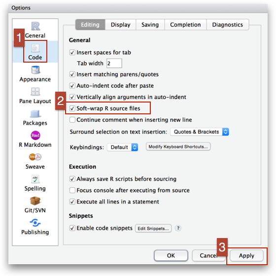
On the left, select “Code” and put a check against “Soft-wrap R source files”. Make sure you click the “Apply” button at the bottom of the Window before saying “OK”.

Interacting with R

Now that we have our interface and directory structure set up, let’s start playing with R! There are two main ways of interacting with R in RStudio: using the console or by using script editor (plain text files that contain your code).

Console window

The console window (in RStudio, the bottom left panel) is the place where R is waiting for you to tell it what to do, and where it will show the results of a command. You can type commands directly into the console, but they will be forgotten when you close the session.

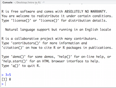
Let’s test it out:

3 + 5

Script editor

Best practice is to enter the commands in the script editor, and save the script. You are encouraged to comment liberally to describe the commands you are running using #. This way, you have a complete record of what you did, you can easily show others how you did it and you can do it again later on if needed.

The Rstudio script editor allows you to ‘send’ the current line or the currently highlighted text to the R console by clicking on the Run button in the upper-right hand corner of the script editor. Alternatively, you can run by simply pressing the Ctrl and Enter keys at the same time as a shortcut.

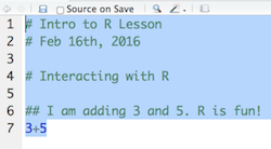
Now let’s try entering commands to the script editor and using the comments character # to add descriptions and highlighting the text to run:

# Intro to R Lesson
# Feb 16th, 2016

# Interacting with R

## I am adding 3 and 5. R is fun!
3+5

You should see the command run in the console and output the result.

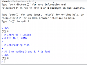
What happens if we do that same command without the comment symbol #? Re-run the command after removing the # sign in the front:

I am adding 3 and 5. R is fun!
3+5

Now R is trying to run that sentence as a command, and it doesn’t work. We get an error in the console “Error: unexpected symbol in “I am” means that the R interpreter did not know what to do with that command.”

Console command prompt

Interpreting the command prompt can help understand when R is ready to accept commands. Below lists the different states of the command prompt and how you can exit a command:

Console is ready to accept commands: >.

If R is ready to accept commands, the R console shows a > prompt.

When the console receives a command (by directly typing into the console or running from the script editor (Ctrl-Enter), R will try to execute it.

After running, the console will show the results and come back with a new > prompt to wait for new commands.

Console is waiting for you to enter more data: +.

If R is still waiting for you to enter more data because it isn’t complete yet, the console will show a + prompt. It means that you haven’t finished entering a complete command. Often this can be due to you having not ‘closed’ a parenthesis or quotation.

Escaping a command and getting a new prompt: esc

If you’re in Rstudio and you can’t figure out why your command isn’t running, you can click inside the console window and press esc to escape the command and bring back a new prompt >.

Exercise

1. Try highlighting only 3 + from your script editor and running it. Find a way to bring back the command prompt > in the console.

Interacting with data in R

R is commonly used for handling big data, and so it only makes sense that we learn about R in the context of some kind of relevant data. Let’s take a few minutes to add files to the folders we created and familiarize ourselves with the data.

Adding files to your working directory

You can access the files we need for this workshop using the links provided below. If you right click on the link, and “Save link as..”. Choose ~/Desktop/Intro-to-R/data as the destination of the file. You should now see the file appear in your working directory. We will discuss these files a bit later in the lesson.

• Download the normalized counts file by right clicking on this link
• Download metadata file using this link

NOTE: If the files download automatically to some other location on your laptop, you can move them to the your working directory using your file explorer or finder (outside RStudio), or navigating to the files in the Files tab of the bottom right panel of RStudio

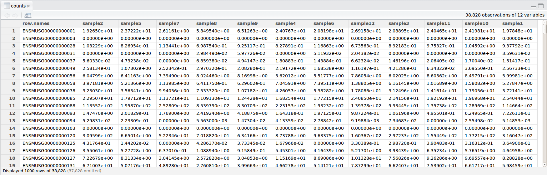
The dataset

In this example dataset, we have collected whole brain samples from 12 mice and want to evaluate expression differences between them. The expression data represents normalized count data obtained from RNA-sequencing of the 12 brain samples. This data is stored in a comma separated values (CSV) file as a 2-dimensional matrix, with each row corresponding to a gene and each column corresponding to a sample.

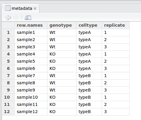
The metadata

We have another file in which we identify information about the data or metadata. Our metadata is also stored in a CSV file. In this file, each row corresponds to a sample and each column contains some information about each sample.

The first column contains the row names, and note that these are identical to the column names in our expression data file above (albeit, in a slightly different order). The next few columns contain information about our samples that allow us to categorize them. For example, the second column contains genotype information for each sample. Each sample is classified in one of two categories: Wt (wild type) or KO (knockout). What types of categories do you observe in the remaining columns?

R is particularly good at handling this type of categorical data. Rather than simply storing this information as text, the data is represented in a specific data structure which allows the user to sort and manipulate the data in a quick and efficient manner. We will discuss this in more detail as we go through the different lessons in R!

Best practices

Before we move on to more complex concepts and getting familiar with the language, we want to point out a few things about best practices when working with R which will help you stay organized in the long run:

• Code and workflow are more reproducible if we can document everything that we do. Our end goal is not just to “do stuff”, but to do it in a way that anyone can easily and exactly replicate our workflow and results. All code should be written in the script editor and saved to file, rather than working in the console.
• The R console should be mainly used to inspect objects, test a function or get help.
• Use # signs to comment. Comment liberally in your R scripts. This will help future you and other collaborators know what each line of code (or code block) was meant to do. Anything to the right of a # is ignored by R. A shortcut for this is Ctrl + Shift + C if you want to comment an entire chunk of text.

This lesson has been developed by members of the teaching team at the Harvard Chan Bioinformatics Core (HBC). These are open access materials distributed under the terms of the Creative Commons Attribution license (CC BY 4.0), which permits unrestricted use, distribution, and reproduction in any medium, provided the original author and source are credited.

• The materials used in this lesson are adapted from work that is Copyright © Data Carpentry (http://datacarpentry.org/). All Data Carpentry instructional material is made available under the Creative Commons Attribution license (CC BY 4.0).