Introduction to R practice
Creating vectors/factors and dataframes
- We are performing RNA-Seq on cancer samples being treated with three different types of treatment (A, B, and P). You have 12 samples total, with 4 replicates per treatment. Write the R code you would use to construct your metadata table as described below.
- Create the vectors/factors for each column (Hint: you can type out each vector/factor, or if you want the process go faster try exploring the
rep()function). - Put them together into a dataframe called
meta. - Use the
rownames()function to assign row names to the dataframe (Hint: you can type out the row names as a vector, or if you want the process go faster try exploring thepaste()function).
Your finished metadata table should have information for the variables
sex,stage,treatment, andmyclevels:sex stage treatment myc sample1 M I A 2343 sample2 F II A 457 sample3 M II A 4593 sample4 F I A 9035 sample5 M II B 3450 sample6 F II B 3524 sample7 M I B 958 sample8 F II B 1053 sample9 M II P 8674 sample10 F I P 3424 sample11 M II P 463 sample12 F II P 5105 - Create the vectors/factors for each column (Hint: you can type out each vector/factor, or if you want the process go faster try exploring the
Subsetting vectors/factors and dataframes
-
Using the
metadata frame from question #1, write out the R code you would use to perform the following operations (questions DO NOT build upon each other):- return only the
treatmentandsexcolumns: - return the
treatmentvalues for samples 5, 7, 9, and 10: - use
subset()to return all data for those samples receiving treatmentP: - use
subset()to return only thestageandtreatmentdata for those samples withmyc> 5000: - remove the
treatmentcolumn from the dataset: - remove samples 7, 8 and 9 from the dataset:
- keep only samples 1-6:
- add a column called
pre_treatmentto the beginning of the dataframe with the values T, F, F, F, T, T, F, T, F, F, T, T (Hint: usecbind()): - change the names of the columns to: “A”, “B”, “C”, “D”:
- return only the
Extracting components from lists
-
Create a new list,
list3with three components, theglengthsvector, the dataframedf, andnumbervalue. Use this list to answer the questions below .list3has the following structure (NOTE: the components of this list are not currently named):[[1]] [1] 4.6 3000.0 50000.0 [[2]] species glengths 1 ecoli 4.6 2 human 3000.0 3 corn 50000.0 [[3]] [1] 8
Write out the R code you would use to perform the following operations (questions DO NOT build upon each other):
- return the second component of the list:
- return
50000.0from the first component of the list: - return the value
humanfrom the second component: - give the components of the list the following names: “genome_lengths”, “genomes”, “record”:
Creating figures with ggplot2
-
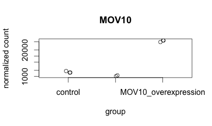
Create the same plot as above using ggplot2 using the provided metadata and counts datasets. The metadata table describes an experiment that you have setup for RNA-seq analysis, while the associated count matrix gives the normalized counts for each sample for every gene. Download the count matrix and metadata using the links provided.
Follow the instructions below to build your plot. Write the code you used and provide the final image.
-
Read in the metadata file using:
meta <- read.delim("Mov10_full_meta.txt", sep="\t", row.names=1) -
Read in the count matrix file using:
data <- read.delim("normalized_counts.txt", sep="\t", row.names=1) -
Create a vector called
expressionthat contains the normalized count values from the row in normalized_counts that corresponds to the MOV10 gene. -
Check the class of this expression vector. You will need to convert this to a numeric vector using
as.numeric(expression) -
Bind that vector to your metadata data frame (
meta) and call the new data framedf. -
Create a ggplot by constructing the plot line by line:
-
Initialize a ggplot with your
dfas input. -
Add the
geom_jitter()geometric object with the required aesthetics which are x and y. -
Color the points based on
sampletype -
Add the
theme_bw()layer -
Add the title “Expression of MOV10” to the plot
-
Change the x-axis label to be blank
-
Change the y-axis label to “Normalized counts”
-
Using
theme()change the following properties of the plot:-
Remove the legend (Hint: use ?theme help and scroll down to legend.position)
-
Change the plot title size to 1.5x the default
-
Change the axis title to 1.5x the default size
-
Change the size of the axis text only on the y-axis to 1.25x the default size
-
-
-
Practice with nested functions (optional)
Let’s derive some nested functions similar to those we will use in our RNA-Seq analysis. The following dataframes, value_table and meta, should be used to address the questions below (you do not actually need to create these dataframes):
value_table
| MX1 | MX2 | MX3 | |
|---|---|---|---|
| KD.2 | -222517.197 | -21756.82 | -16036.035 |
| KD.3 | 17453.907 | -30058.14 | -25837.482 |
| OE.1 | -31247.923 | 73061.38 | 7019.940 |
| OE.2 | -4184.355 | 61994.47 | 1777.858 |
| OE.3 | 147391.709 | 11970.45 | -18663.686 |
| IR.1 | -32247.617 | -27896.01 | 29383.153 |
| IR.2 | 25456.820 | -30714.29 | 19148.752 |
| IR.3 | 99894.656 | -36601.04 | 3207.501 |
meta
| sampletype | MOVexpr | |
|---|---|---|
| KD.2 | MOV10_knockdown | low |
| KD.3 | MOV10_knockdown | low |
| OE.1 | MOV10_overexpression | high |
| OE.2 | MOV10_overexpression | high |
| OE.3 | MOV10_overexpression | high |
| IR.1 | siRNA | normal |
| IR.2 | siRNA | normal |
| IR.3 | siRNA | normal |
-
We would like to count the number of samples which have normal Mov10 expression (
MOVexpr) in themetadataset. Let’s do this in steps:-
Write the R code you would run to return the row numbers of the samples with
MOVexprequal to “normal”: -
Write the R code you would run to determine the number of elements in the
MOVexprcolumn: -
Now, try to combine your first two actions into a single line of code using nested functions to determine the number of elements in the MOVexpr column with expression levels of MOV10 being normal:
-
-
Now we would like to add the
MX1andMX3columns to themetadata frame. Let’s do this in steps:-
Write the R code you would run to extract columns
MX1andMX3from thevalue_tableand to save it to a variablemx(hint: you will need to use thec()function to specify the columns you want to extract): -
Using the
cbind()function, write the R code you would use to add the columns in yourmxvariable to the end of yourmetadataset : -
Now, try to combine your first two actions into a single line of code using nested functions (hint: you do not need to generate the
mxvariable) to add theMX1andMX3columns to themetafile:
-
-
Finally, we would like to extract only those rows from the
metadataset for replicate 2 from all conditions (KD.2, OE.2, IR.2). Let’s do this in steps:-
Write the function you would use to determine the row names of the
metadataset: -
Using the
which()function, write the R code you would run to determine the location of the row nameKD.2in themetadataset: -
Using the which()function, write the R code you would use to determine the location of row namesKD.2,OE.2, andIR.2in themetadataset (use the OR operator () to return multiple locations): - Now, extract the rows from the
metadataset with row namesKD.2,OE.2, andIR.2using a single line of code using nested functions:
-