getwd()[1] "/Users/nos491/Desktop/Intro-to-R-flipped/lessons"Approximate time: 45 minutes
The common misconception is that R is a programming language but in fact it is much more than that. Think of R as an environment for statistical computing and graphics, which brings together a number of features to provide powerful functionality.
The R environment combines:
R is a powerful, extensible environment. It has a wide range of statistics and general data analysis and visualization capabilities.
RStudio is freely available open-source Integrated Development Environment (IDE). RStudio provides an environment with many features to make using R easier and is a great alternative to working on R in the terminal.
![]()
Let’s create a new project directory for our “Introduction to R” lesson today.
File menu and select New Project.New Project window, choose New Directory. Then, choose New Project. Name your new directory Intro-to-R and then “Create the project as subdirectory of:” the Desktop (or location of your choice).Create Project.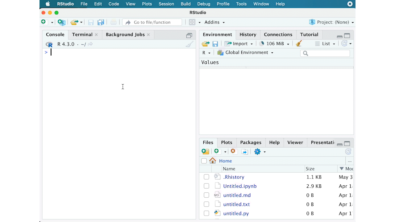
File menu, select Open Project, and choose Intro-to-R.Rproj.File menu and select New File, and select R Script.File menu and select Save As..., type Intro-to-R.R and select Save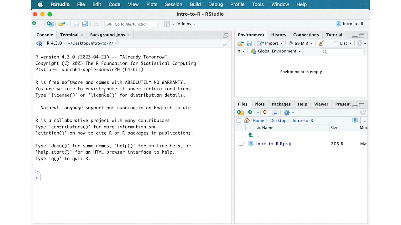
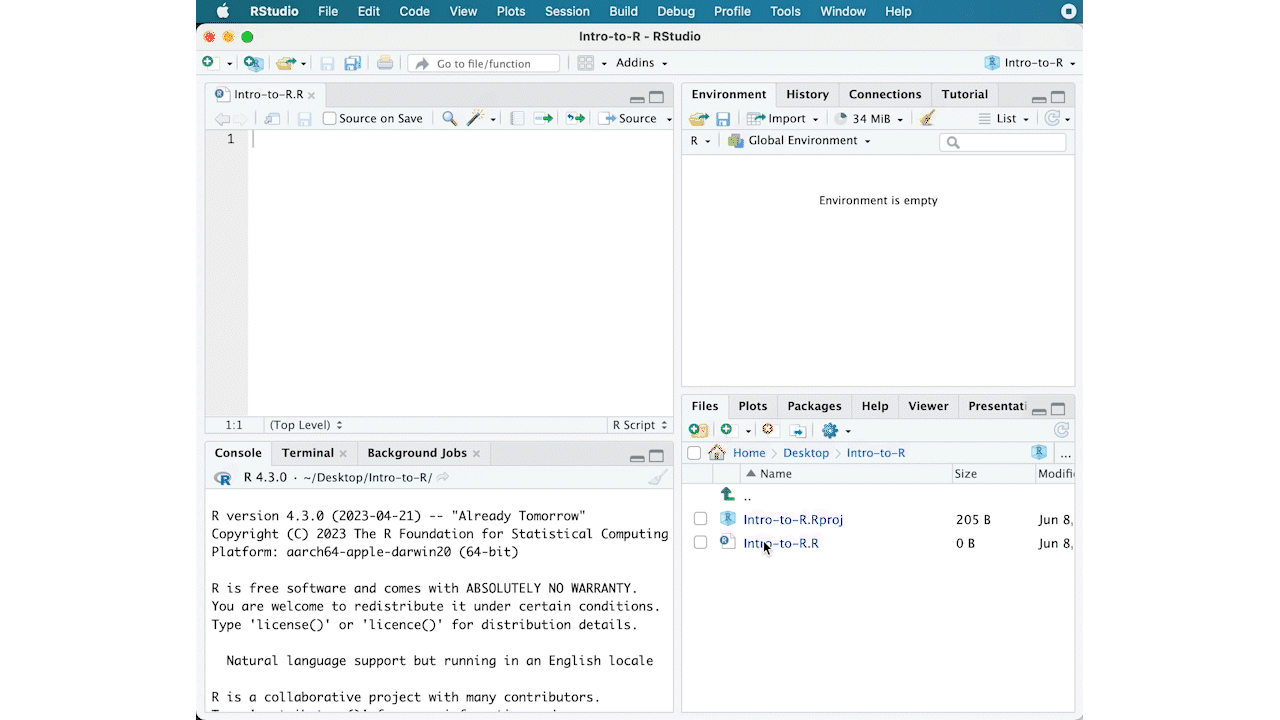
The RStudio interface should now look like the screenshot below.
It is simply a directory that contains everything related your analyses for a specific project. RStudio projects are useful when you are working on context- specific analyses and you wish to keep them separate. When creating a project in RStudio you associate it with a working directory of your choice (either an existing one, or a new one). A . RProj file is created within that directory and that keeps track of your command history and variables in the environment. The . RProj file can be used to open the project in its current state but at a later date.
When a project is (re) opened within RStudio the following actions are taken:
Information adapted from RStudio Support Site
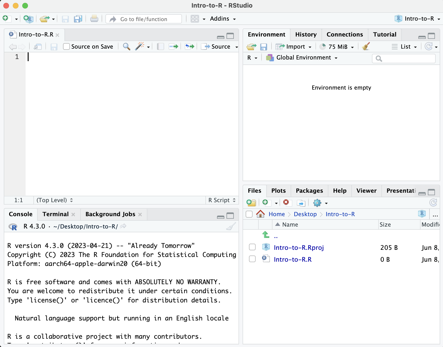
The RStudio interface has four main panels:
Before we organize our working directory, let’s check to see where our current working directory is located by typing into the console:
getwd()[1] "/Users/nos491/Desktop/Intro-to-R-flipped/lessons"Your working directory should be the Intro-to-R folder constructed when you created the project. The working directory is where RStudio will automatically look for any files you bring in and where it will automatically save any files you create, unless otherwise specified.
You can visualize your working directory by selecting the Files tab from the Files/Plots/Packages/Help window.
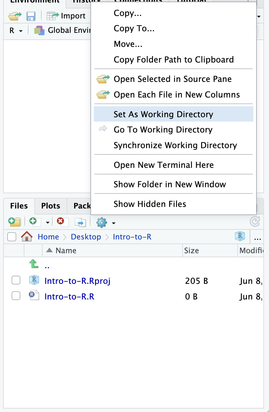
If you wanted to choose a different directory to be your working directory, you could navigate to a different folder in the Files tab, then, click on the More dropdown menu which appears as a Cog and select Set As Working Directory.
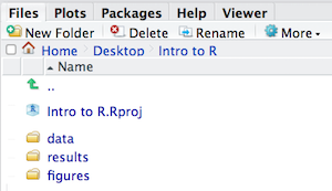
To organize your working directory for a particular analysis, you should separate the original data (raw data) from intermediate datasets. For instance, you may want to create a data/ directory within your working directory that stores the raw data, and have a results/ directory for intermediate datasets and a figures/ directory for the plots you will generate.
Let’s create these three directories within your working directory by clicking on New Folder within the Files tab.
When finished, your working directory should look like:
This is more of a housekeeping task. We will be writing long lines of code in our script editor and want to make sure that the lines “wrap” and you don’t have to scroll back and forth to look at your long line of code.
Click on “Code” at the top of your RStudio screen and select “Soft Wrap Long Lines” in the pull down menu.
Now that we have our interface and directory structure set up, let’s start playing with R! There are two main ways of interacting with R in RStudio: using the console or by using script editor (plain text files that contain your code).
The console window (in RStudio, the bottom left panel) is the place where R is waiting for you to tell it what to do, and where it will show the results of a command. You can type commands directly into the console, but they will be forgotten when you close the session.
Let’s test it out:
3 + 5[1] 8Best practice is to enter the commands in the script editor, and save the script. You are encouraged to comment liberally to describe the commands you are running using #. This way, you have a complete record of what you did, you can easily show others how you did it and you can do it again later on if needed.
The Rstudio script editor allows you to ‘send’ the current line or the currently highlighted text to the R console by clicking on the Run button in the upper-right hand corner of the script editor.
Now let’s try entering commands to the script editor and using the comments character # to add descriptions and highlighting the text to run:
# Intro to R Lesson
# Feb 16th, 2016

# Interacting with R

## I am adding 3 and 5. R is fun!
3 + 5
[1] 8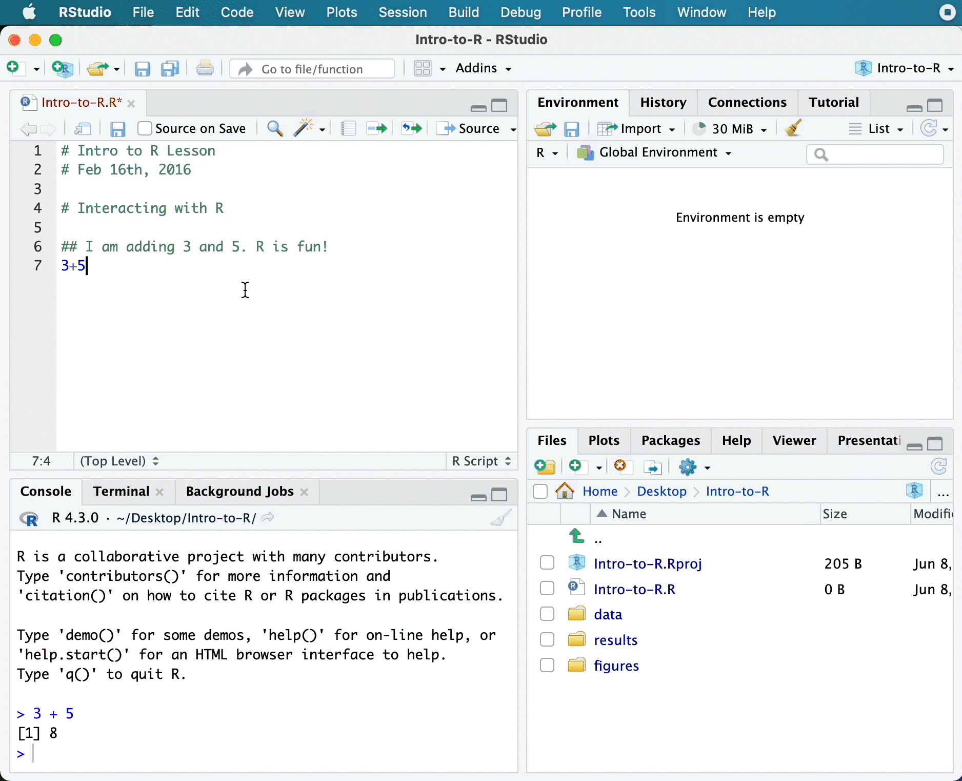
Alternatively, you can run by simply pressing the Ctrl and Return/Enter keys at the same time as a shortcut.
You should see the command run in the console and output the result.
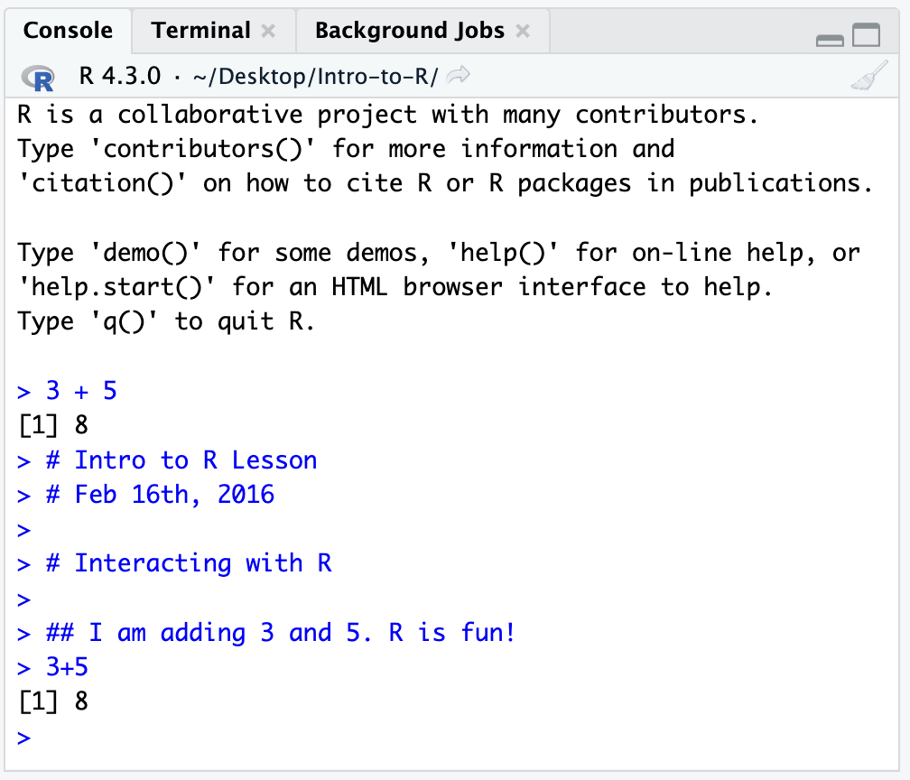
What happens if we do that same command without the comment symbol #? Re-run the command after removing the # sign in the front:
I am adding 3 and 5. R is fun!
3+5
Now R is trying to run that sentence as a command, and it doesn’t work. We get an error in the console
Error: unexpected symbol in “I am”
This means that the R interpreter did not know what to do with that command
Interpreting the command prompt can help understand when R is ready to accept commands. Below lists the different states of the command prompt and how you can exit a command:
Console is ready to accept commands: >.
If R is ready to accept commands, the R console shows a > prompt.
When the console receives a command (by directly typing into the console or running from the script editor (Ctrl-Enter), R will try to execute it.
After running, the console will show the results and come back with a new > prompt to wait for new commands.
Console is waiting for you to enter more data: +.
If R is still waiting for you to enter more data because it isn’t complete yet, the console will show a + prompt. It means that you haven’t finished entering a complete command. Often this can be due to you having not ‘closed’ a parenthesis or quotation.
Escaping a command and getting a new prompt: esc
If you’re in Rstudio and you can’t figure out why your command isn’t running, you can click inside the console window and press esc to escape the command and bring back a new prompt >.
In addition to some of the shortcuts described earlier in this lesson, we have listed a few more that can be helpful as you work in RStudio.
| key | action |
|---|---|
| Ctrl+Enter | Run command from script editor in console |
| ESC | Escape the current command to return to the command prompt |
| Ctrl+1 | Move cursor from console to script editor |
| Ctrl+2 | Move cursor from script editor to console |
| Tab | Use this key to complete a file path |
| Ctrl+Shift+C | Comment the block of highlighted text |
3 + from your script editor and running it. Find a way to bring back the command prompt > in the console.Now that we know how to talk with R via the script editor or the console, we want to use R for something more than adding numbers. To do this, we need to know more about the R syntax.
The main “parts of speech” in R (syntax) include:
# and how they are used to document function and its content<-= for arguments in functionsNOTE: indentation and consistency in spacing is used to improve clarity and legibility
We will go through each of these “parts of speech” in more detail, starting with the assignment operator.
To do useful and interesting things in R, we need to assign values to variables using the assignment operator, <-. For example, we can use the assignment operator to assign the value of 3 to x by executing:
x <- 3The assignment operator (<-) assigns values on the right to variables on the left.
In RStudio, typing Alt + - (push Alt at the same time as the - key, on Mac type option + -) will write <- in a single keystroke.
A variable is a symbolic name for (or reference to) information. Variables in computer programming are analogous to “buckets”, where information can be maintained and referenced. On the outside of the bucket is a name. When referring to the bucket, we use the name of the bucket, not the data stored in the bucket.
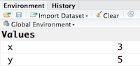
In the example above, we created a variable or a ‘bucket’ called x. Inside we put a value, 3.
Let’s create another variable called y and give it a value of 5.
y <- 5When assigning a value to an variable, R does not print anything to the console. You can force to print the value by using parentheses or by typing the variable name.
y[1] 5You can also view information on the variable by looking in your Environment window in the upper right-hand corner of the RStudio interface.
Now we can reference these buckets by name to perform mathematical operations on the values contained within. What do you get in the console for the following operation:
x + y[1] 8Try assigning the results of this operation to another variable called number.
number <- x + yx to 5. What happens to number?y to contain the value 10. What do you need to do, to update the variable number?Variables can be given almost any name, such as x, current_temperature, or subject_id. However, there are some rules / suggestions you should keep in mind:
2x is not valid but x2 is)if, else, for, see here for a complete list). In general, even if it’s allowed, it’s best to not use other function names (e.g., c, T, mean, data) as variable names. When in doubt check the help to see if the name is already in use..) within a variable name as in my.dataset. There are many functions in R with dots in their names for historical reasons, but because dots have a special meaning in R (for methods) and other programming languages, it’s best to avoid them.genome_length is different from Genome_length)R is commonly used for handling big data, and so it only makes sense that we learn about R in the context of some kind of relevant data. Let’s take a few minutes to add files to the folders we created and familiarize ourselves with the data.
You can access the files we need for this workshop using the links provided below. If you right click on the link, and “Save link as..”. Choose ~/Desktop/Intro-to-R/data as the destination of the file. You should now see the file appear in your working directory. We will discuss these files a bit later in the lesson.
NOTE: If the files download automatically to some other location on your laptop, you can move them to the your working directory using your file explorer or finder (outside RStudio), or navigating to the files in the
Filestab of the bottom right panel of RStudio
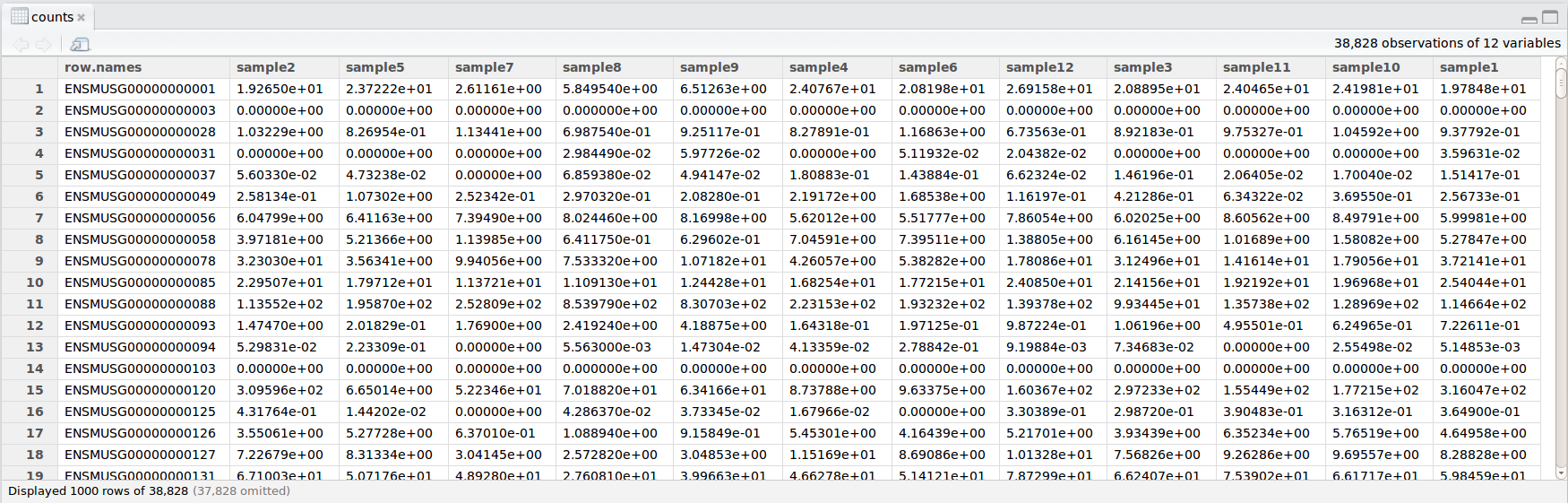
In this example dataset, we have collected whole brain samples from 12 mice and want to evaluate expression differences between them. The expression data represents normalized count data obtained from RNA-sequencing of the 12 brain samples. This data is stored in a comma separated values (CSV) file as a 2-dimensional matrix, with each row corresponding to a gene and each column corresponding to a sample.
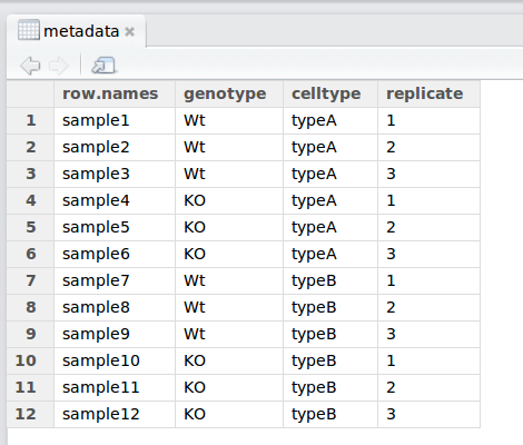
We have another file in which we identify information about the data or metadata. Our metadata is also stored in a CSV file. In this file, each row corresponds to a sample and each column contains some information about each sample.
The first column contains the row names, and note that these are identical to the column names in our expression data file above (albeit, in a slightly different order). The next few columns contain information about our samples that allow us to categorize them. For example, the second column contains genotype information for each sample. Each sample is classified in one of two categories: Wt (wild type) or KO (knockout). What types of categories do you observe in the remaining columns?
R is particularly good at handling this type of categorical data. Rather than simply storing this information as text, the data is represented in a specific data structure which allows the user to sort and manipulate the data in a quick and efficient manner. We will discuss this in more detail as we go through the different lessons in R!
We will be using the results of the functional analysis to learn about packages/functions from the Tidyverse suite of integrated packages. These packages are designed to work together to make common data science operations like data wrangling, tidying, reading/writing, parsing, and visualizing, more user-friendly.
Before we move on to more complex concepts and getting familiar with the language, we want to point out a few things about best practices when working with R which will help you stay organized in the long run:
# signs to comment. Comment liberally in your R scripts. This will help future you and other collaborators know what each line of code (or code block) was meant to do. Anything to the right of a # is ignored by R. A shortcut for this is Ctrl+Shift+C if you want to comment an entire chunk of text.