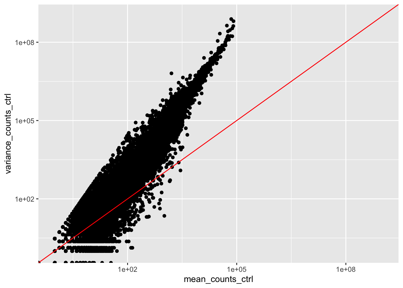
Evaluate the relationship between mean and variance for the control replicates (Irrel_kd samples). Note the differences or similarities in the plot compared to the one using the overexpression replicates.
mean_counts_ctrl <-apply(data[,1:3], 1, mean) # select column 1 to 3, which correspond to Irrel_kd samplesvariance_counts_ctrl <-apply(data[,1:3], 1, var)df_ctrl <-data.frame(mean_counts_ctrl, variance_counts_ctrl)ggplot(df_ctrl) +geom_point(aes(x = mean_counts_ctrl, y = variance_counts_ctrl)) +# plot mean vs variancescale_y_log10(limits =c(1,1e9)) +scale_x_log10(limits =c(1,1e9)) +geom_abline(intercept =0, slope =1, color ="red") # add a line for x = y (slope = 1)
The plot of mean and variance for the control replicates is similar to that of overexpression replicates shown in the lesson.
Exercise 2
An RNA-seq experiment was conducted on mice forebrain to evaluate the effect of increasing concentrations of a treatment. For each of the five different concentrations we have n = 5 mice for a total of 25 samples. If we observed little to no variability between replicates, what might this suggest about our samples?
The lack of variability between replicates suggests that we are possibly dealing with technical replicates. With true biological replicates we expect some amount of variability. If you have technical replicates, you do not want to be using DESeq2 because we will be using the NB to account for overdispersion, which doesn’t exist.
What type of mean-variance relationship would you expect to see for this dataset?
mean == variance. A Poisson would be more appropriate.
Source Code
---title: "RNA-seq count data distribution - Answer key"---```{r data_setup}#| echo: false# load libraries needed to render this lessonlibrary(ggplot2)# load objects needed to render this lessondata <- readRDS("./data/intermediate_txi_counts.RDS")```# Exercise 1**Evaluate the relationship between mean and variance for the control replicates (Irrel_kd samples). Note the differences or similarities in the plot compared to the one using the overexpression replicates.**```{r}mean_counts_ctrl <-apply(data[,1:3], 1, mean) # select column 1 to 3, which correspond to Irrel_kd samplesvariance_counts_ctrl <-apply(data[,1:3], 1, var)df_ctrl <-data.frame(mean_counts_ctrl, variance_counts_ctrl)ggplot(df_ctrl) +geom_point(aes(x = mean_counts_ctrl, y = variance_counts_ctrl)) +# plot mean vs variancescale_y_log10(limits =c(1,1e9)) +scale_x_log10(limits =c(1,1e9)) +geom_abline(intercept =0, slope =1, color ="red") # add a line for x = y (slope = 1)```The plot of mean and variance for the control replicates is similar to that of overexpression replicates shown in the lesson.# Exercise 2**An RNA-seq experiment was conducted on mice forebrain to evaluate the effect of increasing concentrations of a treatment. For each of the five different concentrations we have n = 5 mice for a total of 25 samples. If we observed little to no variability between replicates, what might this suggest about our samples?**The lack of variability between replicates suggests that we are possibly dealing with technical replicates. With true biological replicates we expect some amount of variability. If you have technical replicates, you do not want to be using DESeq2 because we will be using the NB to account for overdispersion, which doesn't exist.**What type of mean-variance relationship would you expect to see for this dataset?**mean == variance. A Poisson would be more appropriate.