Learning Objectives
- Discussing features of Rmarkdown
- Creating reports using knitr
Reproducible reports in R
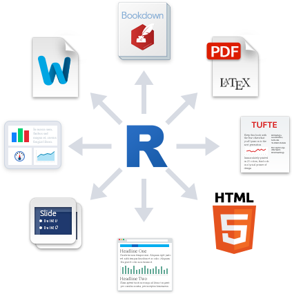
So far, any code that we have written in R has been in the form of an R script (.R). Any figures that we generated, were either plotted to the RStudio device and/or exported to file. What if we wanted to communicate this with our collaborators? Wouldn’t it be nice to be able to share the code along with tables, figures, and text describing the interpretation? Thankfully, in RStudio there is a way to compile all of that information into a report by using the knitr package and a simple text-markup language called RMarkdown. The combination of these two things allow users to combine code and stylized text to output information in various formats including HTML, PDF, MS_Word, ODT, RTF, Markdown, and Github flavored Markdown documents.
Markdown
Before we get started with RMarkdown, we have a short digression on Markdown, a text-to-HTML conversion tool for web writers. Simply put, Markdown is a way to style text on the web. It is mostly just regular text with a few non-alphabetic characters thrown in, like # or * to help with stylistic details.
NOTE: You can use Markdown most places around GitHub. This lesson is all written in Markdown!
Some commonly used formatting options are listed below:
- The
#character is used to denote a header
# This is a Heading1 tag
## This is a Heading2 tag
This is a Heading1 tag
This is a Heading2 tag
- The asterik
*and underscore_characters are used to add emphasis to select words
*This text will be italicized.*
_This will also be italicized._

**This text will be bold.**
__This will also be bold.__

_You **can** combine them!_
This text will be italicized. This will also be italicized.
This text will be bold. This will also be bold.
You can combine them!
- Lists can be displayed using bullet points
* Item 1
* Item 2
  * Item 2a
  * Item 2b
- Item 1
- Item 2
- Item 2a
- Item 2b
- Lists can be ordered with numbers
1. Item 1
1. Item 2
   1. Item 2a
   1. Item 2b
- Item 1
- Item 2
- Item 2a
- Item 2b
This is really just scratching the surface of what you can do in Markdown. There are also ways in which you can include images, links, block quotes and code (inline and code chunks). In the interest of time, we won’t go into detail here but we will point you to some very useful resources.
Resources for Markdown
NOTE: If you are working with Markdown most text editors will automatically syntax highlight but there are also various Markdown specific editors which allow you to see see the rendered version of your text as you type (i.e. MacDown for Macs, MarkdownPad for Windows).
RMarkdown
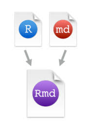
Markdown has proved so useful that many different coding groups adopted it, but also adding there own ‘flavours’. RStudio implements something called “R-flavoured markdown” (or RMarkdown) which has various features that we describe below. Rather than creating a .R script, you would create an .Rmd file which would contain code and stylized plain text using some of the options described in the Markdown section.
Introduction to knitr
knitr, developed by Yihui Xie, is an R package designed for report generation within RStudio. ![]() It takes an RMarkdown file (.Rmd) and enables dynamic generation of multiple file formats from an RMarkdown file, including HTML and PDF documents. As RMarkdown grows as an acceptable reproducible manuscript format, using knitr to generate a report summary is becoming common practice. Knit report generation is now integrated into RStudio, and can be accessed using the GUI or console.
It takes an RMarkdown file (.Rmd) and enables dynamic generation of multiple file formats from an RMarkdown file, including HTML and PDF documents. As RMarkdown grows as an acceptable reproducible manuscript format, using knitr to generate a report summary is becoming common practice. Knit report generation is now integrated into RStudio, and can be accessed using the GUI or console.
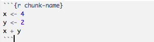
Code chunks
The basic idea of knitr (along with RMarkdown) is that you can write your analysis workflow in plain text and intersperse chunks of code delimited with a special marker (```). Backticks (`) commonly indicate code and are also used on GitHub. Each chunk should be given a unique name. knitr isn’t very picky how you name the code chunks, but we recommend using snake_case for the names whenever possible.
Additionally, you can write inline R code enclosed by single backticks (`) containing a lowercase r (like ``` code chunks). This allows for variable returns outside of code chunks, and is extremely useful for making report text more dynamic. For example, you can print the current date inline with this syntax: ` r Sys.Date() ` (no spaces).
Per chunk options
knitr provides a lot of customization options for code chunks, which are written in the form of tag=value.
There is a comprehensive list of all the options available, however when starting out this can be overwhelming. Here, we provide a short list of some options commonly use in chunks:
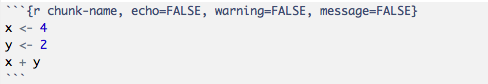
echo = TRUE: whether to include R source code in the output fileeval = TRUE: whether to evaluate/execute the codeinclude = TRUE: whether to include the chunk output in the final output document; if include=FALSE, nothing will be written into the output document, but the code is still evaluated and plot files are generated if there are any plots in the chunk, so you can manually insert figureswarning = TRUE: whether to preserve warnings in the output like we run R code in a terminal (if FALSE, all warnings will be printed in the console instead of the output document)message = TRUE: whether to preserve messages emitted by message() (similar to warning)results = "asis": output as-is, i.e., write raw results from R into the output document
There are also a few options commonly used for plots to easily resize images:
fig.height = 6fig.width = 4
Global options
knitr allows for global options to be set on all chunks in an RMarkdown file. These are options that should be placed inside your setup chunk at the top of your RMarkdown document.
opts_chunk$set(
    autodep = TRUE,
    cache = TRUE,
    cache.lazy = TRUE,
    dev = c("png", "pdf", "svg"),
    error = TRUE,
    fig.height = 6,
    fig.retina = 2,
    fig.width = 6,
    highlight = TRUE,
    message = FALSE,
    prompt = TRUE,
    tidy = TRUE,
    warning = FALSE)
The setup chunk
The setup chunk is a special knitr chunk that should be placed at the start of the document. We recommend storing all the user-defined parameters in the setup chunk that are required for successful knitting. Also you could include all library() loads required for the script and other load() requests for external files here.
{r setup, include=FALSE}

#=================
# Load packages (load all the packages here at the beginning)
#=================
library(xtable) ## for making awesome tables
library(ggplot2) ## for plotting

# Set some basic options. You usually do not want your code, messages,
# warnings etc to show in your actual manuscript however for the first
# run or two these will be set on.

knitr::opts_chunk$set(warning=TRUE,
            message=TRUE,
            echo=TRUE,
            cache = FALSE,
            tidy = FALSE, ## remove the auto-formatting
            error=TRUE)
NOTE: An additional cool trick is that you can save
opts_chunk$setsettings in~/.Rprofileand these knitr options will apply to all of your RMarkdown documents.
Figures
A neat feature of knitr is how much simpler it makes generating figures. You can simply return a plot in a chunk, and knitr will automatically write the files to disk, in an organized subfolder. By specifying options in the setup chunk, you can have R automatically save your plots in multiple file formats at once, including PNG, PDF, and SVG. A single chunk can support multiple plots, and they will be arranged in squares below the chunk in RStudio.
Tables
knitr includes a simple but powerful function for generating stylish tables in a knit report named kable(). Here’s an example using R’s built-in mtcars dataset:
help("kable", "knitr")
mtcars %>%
    head %>%
    kable
| mpg | cyl | disp | hp | drat | wt | qsec | vs | am | gear | carb | |
|---|---|---|---|---|---|---|---|---|---|---|---|
| Mazda RX4 | 21.0 | 6 | 160 | 110 | 3.90 | 2.620 | 16.46 | 0 | 1 | 4 | 4 |
| Mazda RX4 Wag | 21.0 | 6 | 160 | 110 | 3.90 | 2.875 | 17.02 | 0 | 1 | 4 | 4 |
| Datsun 710 | 22.8 | 4 | 108 | 93 | 3.85 | 2.320 | 18.61 | 1 | 1 | 4 | 1 |
| Hornet 4 Drive | 21.4 | 6 | 258 | 110 | 3.08 | 3.215 | 19.44 | 1 | 0 | 3 | 1 |
| Hornet Sportabout | 18.7 | 8 | 360 | 175 | 3.15 | 3.440 | 17.02 | 0 | 0 | 3 | 2 |
| Valiant | 18.1 | 6 | 225 | 105 | 2.76 | 3.460 | 20.22 | 1 | 0 | 3 | 1 |
Generating the report
knit() (recommended)
help("knit", "knitr")
Once we’ve finished creating an RMarkdown file containing code chunks, we finally need to knit the report. When executing knit() on a document, by default this will generate an HTML report. If you would prefer a different document format, this can be specified in the YAML header with the output: parameter:
- html_document
- pdf_document
- github_document
RStudio now supports a number of formats, each with their own customization options. Consult their website for more details.
render() (advanced)
help("render", "rmarkdown")
The knit() command works great if you only need to generate a single document format. RMarkdown also supports a more advanced function named rmarkdown::render(), allows for output of multiple document formats. To accomplish this, we recommend saving a special file named _output.yaml in your project root.
rmarkdown::html_document:
    code_folding: hide
    df_print: kable
    highlight: pygments
    number_sections: false
    toc: true
rmarkdown::pdf_document:
    number_sections: false
    toc: true
    toc_depth: 1
NOTE: PDF rendering is sometimes problematic, especially when running R remotely, like on the O2 cluster. If you run into problems, it’s likely an issue related to pandoc.
Working directory behavior
knitr redefines the working directory of an RMarkdown file in a manner that can be confusing. If you’re working in RStudio with an RMarkdown file that is not at the same location as the current R working directory (
getwd()), you can run into problems with broken file paths. Suppose you have RStudio open without a project loaded, the working directory is usually set to your home directory. Now, if you load an RMarkdown file from the desktop at~/Users/myserame/Desktop, knitr will set the working directory within chunks to be relative to the desktop. We advise against coding paths in a script to only work with knitr and not base R.A simple way to resolve this issue is by creating an R project for the analysis, and saving all RMarkdown files at the top level, to avoid running into unexpected problems related to this behavior.
Convert an R script to an RMarkdown knit report
Now that we know some of the basics of RMarkdown, let’s convert our Mov10 DE analysis script into an RMarkdown report!
- Download the .Rmd file
- Open up your DEanalysis R project in Rstudio.
- Move your RMarkdown file into the project working directory.
- Open up the .Rmd file and Knit the report.
Download to data folder https://tinyurl.com/download-data-DE
Download to meta folder https://tinyurl.com/download-meta-DE
Once the report has been knit, it should open up in a separate window. If not, you will now see an html file in your workindg directory (de_script_toknit.html) which you can open in a web browser. This report contains some of the commands we ran in Session III. This report is a great template but it can use a few tweaks to make it a bit more aesthetically pleasing.
- Add a title to your report
- Only the first code chunk has a name. Go through and add names to the remaining code chunks.
- Loading the libraries is very verbose and we do no need this output in our final report. To suppress this messaging you will need to set the code chunk options
warning=FALSEandmessage=FALSE. - Remove the verbosity from the DESeq code chunk as well.
- For the QC section we are ony really interested in displaying figures. To hide the code in the report the code chunk option
echo=FALSE. Do the same for the Volcano Plot and Heatmap chunks. - Separate the QC code chunk into two code chunks one for PCA and one for the heatmap. Add subheadings for each chunk and be sure the code is not displayed for either.
- Take a look at the “Summarizing and Visualizing Results” section to see how we have incorporated inline R code
- Remove the warnings from the Volcano Plot code chunk and change the width of the figure output using
fig.width=12. - Separate the code for the last set of heatmaps into OE and KD. Add a sub-heading for each.