Approximate time: 30 minutes
Learning Objectives:
- Understand the general steps leading to generation of the count matrix
Single-cell RNA-seq: raw sequencing data to counts
Single-cell RNA-seq (scRNA-seq) is an exciting and cutting-edge method for analyzing differences in cellular gene expression, particularly for tissue heterogeneity analyses, lineage tracing, and cell population dynamics.
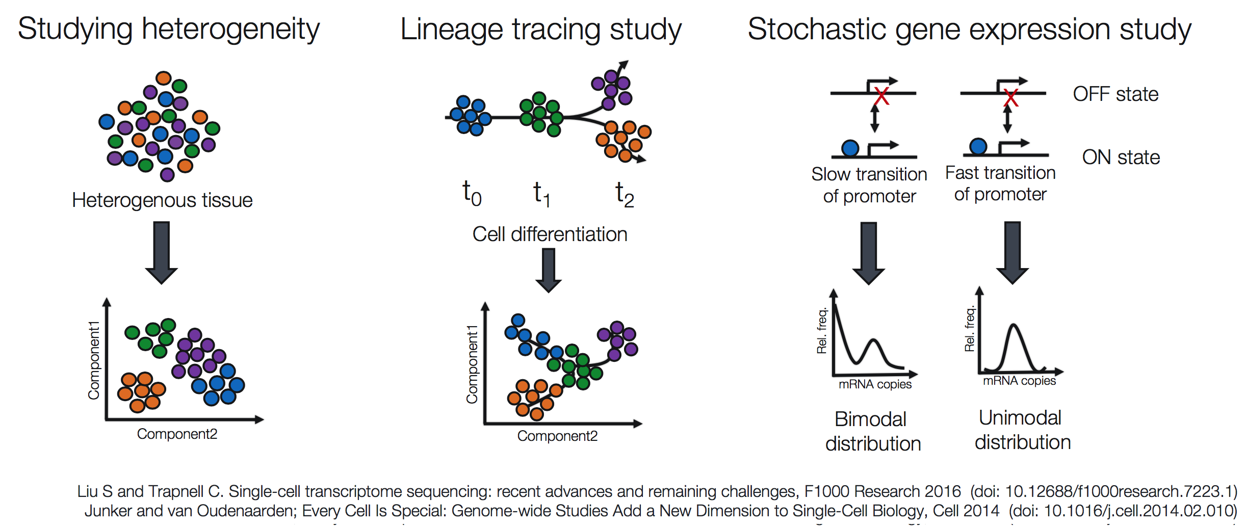
The complexity of scRNA-seq data, which is generally characterized as a large volume of data, representing thousands of cells, and by a low depth of sequencing per cell, resulting in a large number of genes without any corresponding reads (zero inflation), makes analysis of the data more involved than bulk RNA-seq. In addition, the analysis goals can vary depending whether the goal is marker identification, lineage tracing, or some other custom analysis. Therefore, tools specific for scRNA-seq and the different methods of library preparation are needed.
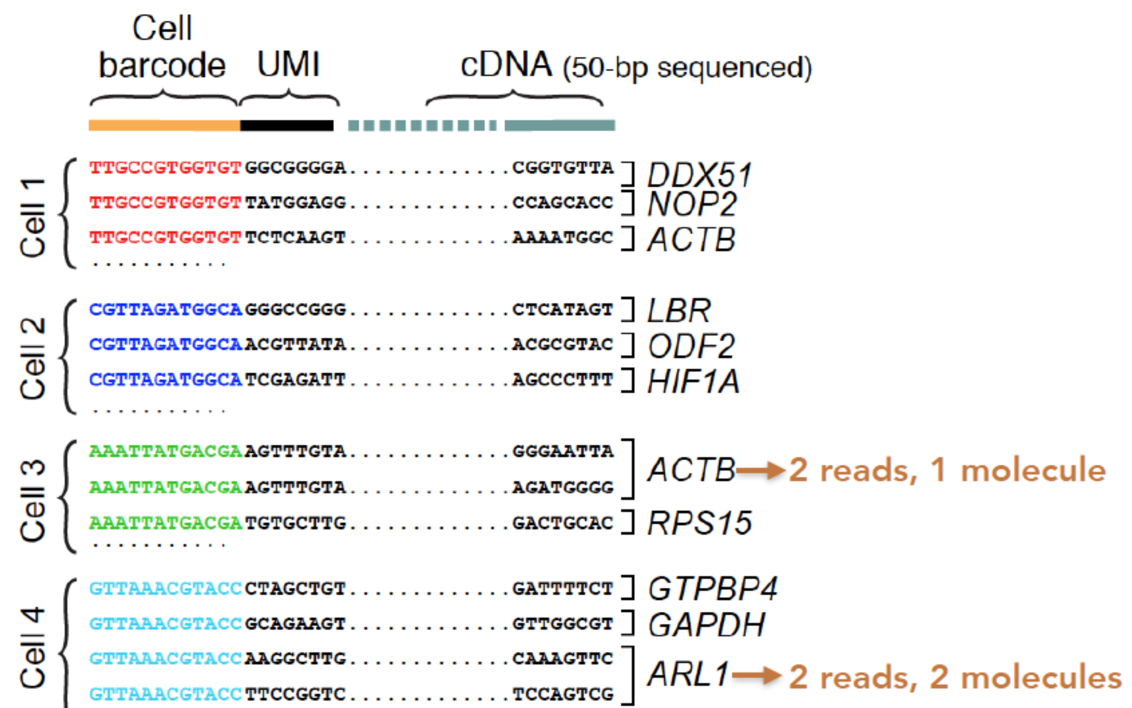
The analysis workflow for scRNA-seq is generally similar for the differing scRNA-seq methods, but some specifics, such as the parsing of the UMIs, cell IDs, and sample IDs, will differ between them. For example, below is a schematic of the inDrop sequence reads:
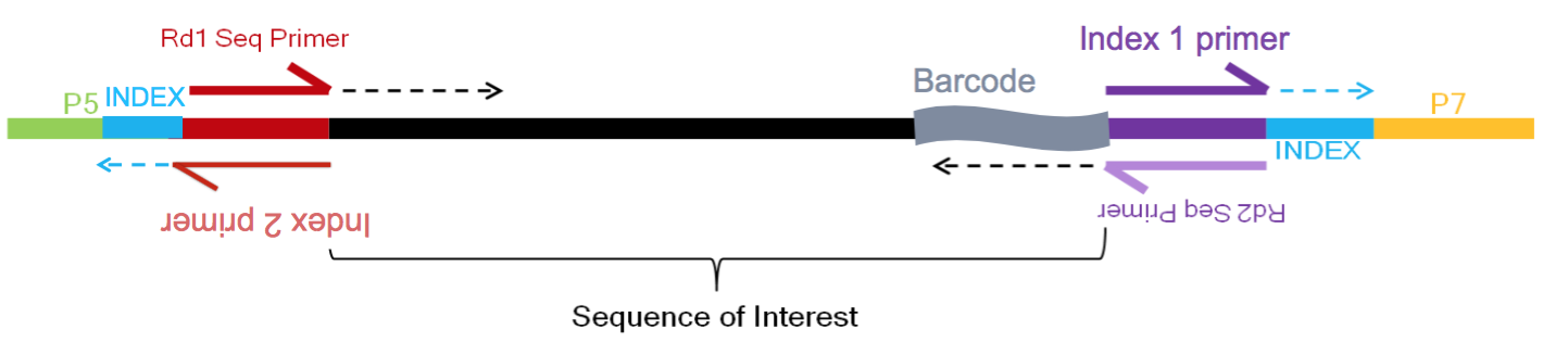
Image credit: Sarah Boswell, Director of the Single Cell Sequencing Core at HMS
While the 10X sequence reads have the UMI and barcodes placed differently:
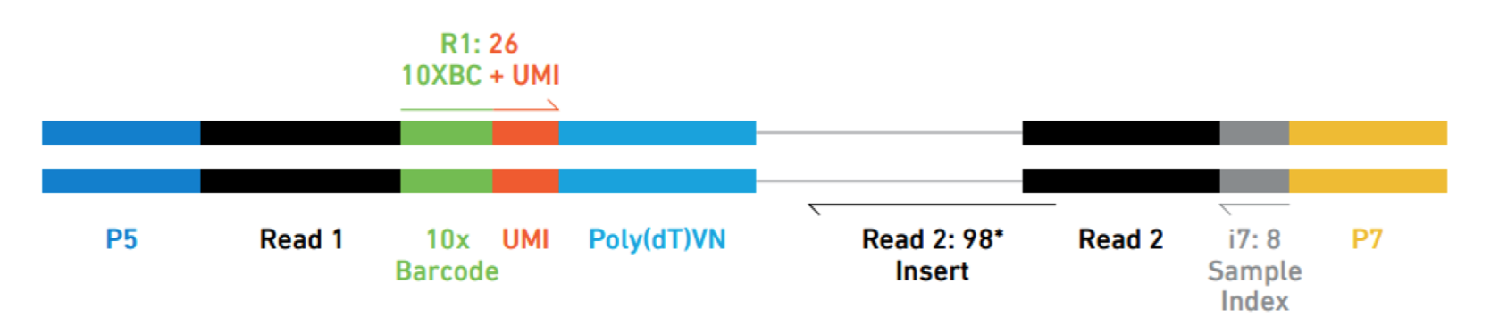
Image credit: Sarah Boswell, Director of the Single Cell Sequencing Core at HMS
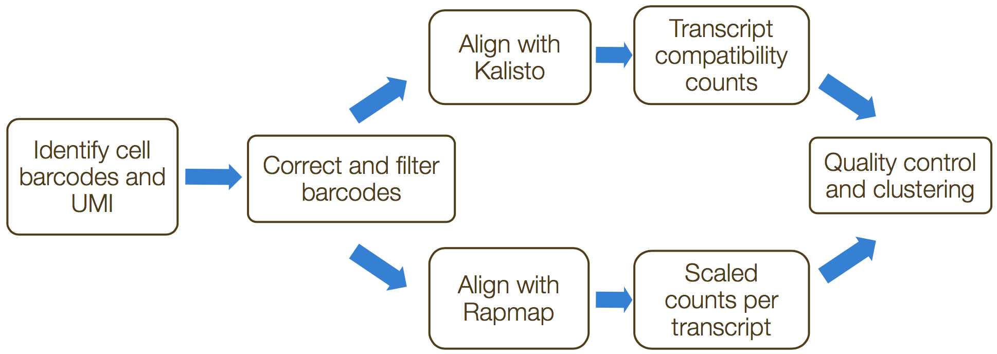
The scRNA-seq method will determine the how to parse the barcodes and UMIs from the sequencing reads. So, although a few of the specific steps will slightly differ, the overall workflow will generally follow the same steps regardless of method. The general workflow is shown below:
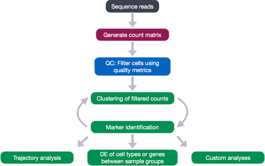
The scRNA-seq method-specific steps are required for the generation of the count matrix, and we will cover what is involved in this later, but after this step, the same methods can be utilized. After generating the count matrix, the raw counts will be assessed to filter out poor quality cells with a low number of genes or UMIs, high mitochondrial gene expression indicative of dying cells, or low number of genes per UMI. After removing the poor quality cells, the cells are clustered based on similarities in transcriptional activity, with the idea that the different cell types separate into the different clusters. After clustering, we can explore genes that are markers for different clusters, which can help identify the cell type of each cluster. Finally, after identification of cell types, there are various types of analyses that can be performed depending on the goal of the experiment.
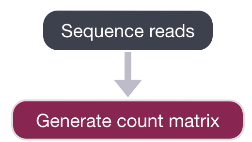
We are going to start by discussing the first part of this workflow, which is generating the count matrix from the raw sequencing data.
The sequencing facility will either output the raw sequencing data as BCL format or FASTQ. If the reads are in BCL format, then we will need to convert into FASTQ format. There is a useful tool on O2 called bcl2fastq that can easily perform this conversion. We do not demultiplex at this step in the workflow. You may have sequenced 6 samples, but the reads for all samples may be present all in the same BCL or FASTQ file.
The generation of the count matrix from the raw sequencing data will go through the following steps for many of the scRNA-seq methods.
’umis provides tools for estimating expression in RNA-seq data which performs sequencing of end tags of transcript, and incorporate molecular tags to correct for amplification bias.’ The steps in this process include the following:
- Formatting reads and filtering noisy cellular barcodes
- Demultiplexing the samples
- Pseudo-mapping to cDNAs
- Counting molecular identifiers
1. Formatting reads and filtering noisy cellular barcodes
The FASTQ files can then be used to parse out the cell barcodes, UMIs, and sample barcodes. Many of the cellular barcodes will match a low number of reads (< 1000 reads) due to encapsulation of free floating RNA from dying cells, small cells, or set of cells that failed for some reason. These excess barcodes need to be filtered out of the sequence data prior to read alignment.
‘All non-biological segments of the sequenced reads for the sake of mapping. While also keeping this information for later use. We consider non-biological information such as Cellular Barcode and Molecular Barcode. To later be able to extract the optional CB and the MB these are put in the read header, with the following format.’
@HWI-ST808:130:H0B8YADXX:1:1101:2088:2222:CELL_GGTCCA:UMI_CCCT
AGGAAGATGGAGGAGAGAAGGCGGTGAAAGAGACCTGTAAAAAGCCACCGN
+
@@@DDBD>=AFCF+<CAFHDECII:DGGGHGIGGIIIEHGIIIGIIDHII#
‘Not all cellular barcodes identified will be real. Some will be low abundance barcodes that do not represent an actual cell. Others will be barcodes that don’t come from a set of known barcodes.’ Unknown barcodes will be dropped, with an argument to specify the number of mismatches acceptable.’
2. Demultiplexing sample reads
The next step of the process is to demultiplex the samples, if sequencing more than a single sample. This is the one step of this process not handled by the ‘umis’ tools. We would need to parse the reads to determine the sample barcode associated with each cell.
3. Pseudo-mapping to cDNAs
‘This is done by pseudo-aligners, either Kallisto or RapMap. The SAM (or BAM) file output from these tools need to be saved.’
4. Counting molecular identifiers
‘The final step is to infer which cDNA was the origin of the tag a UMI was attached to. We use the pseudo-alignments to the cDNAs, and consider a tag assigned to a cDNA as a partial evidence for a (cDNA, UMI) pairing. For actual counting, we only count unique UMIs for (gene, UMI) pairings with sufficient evidence.’
At this point of the workflow, the duplicate UMIs will be collapsed for the counting of the identifiers.
Now we have our count matrix containing the counts per gene for each cell, which we can use to explore our data for quality information.
This lesson has been developed by members of the teaching team at the Harvard Chan Bioinformatics Core (HBC). These are open access materials distributed under the terms of the Creative Commons Attribution license (CC BY 4.0), which permits unrestricted use, distribution, and reproduction in any medium, provided the original author and source are credited.