Approximate time: 30 minutes
Count modeling and Hypothesis testing
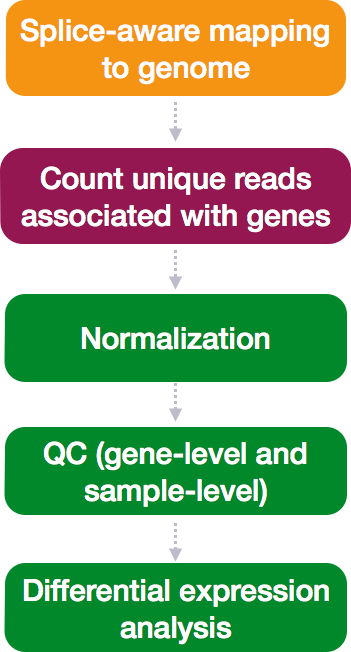
Once the count data is filtered, the next step is to perform the differential expression analysis.
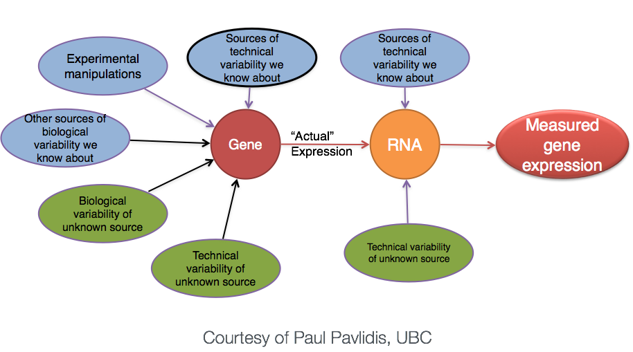
Internally, DESeq2 is performing a number of steps but here we will focus on describing the count modeling and hypothesis testing. Modeling is a mathematically formalized way to approximate how the data behaves given a set of parameters.
Characteristics of RNA-seq count data
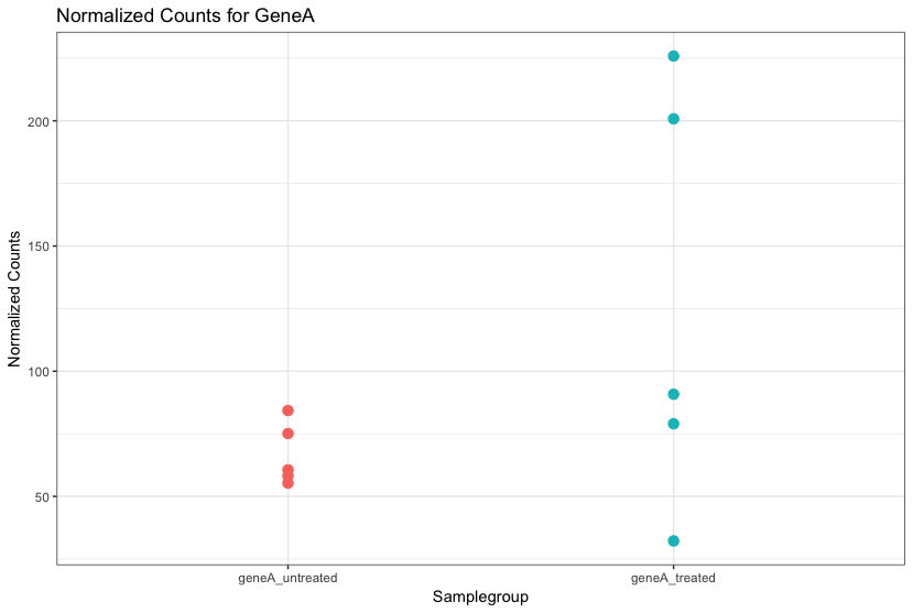
To determine the appropriate statistical model, we need information about the distribution of counts. To get an idea about how RNA-seq counts are distributed, we can plot the counts for a single sample:
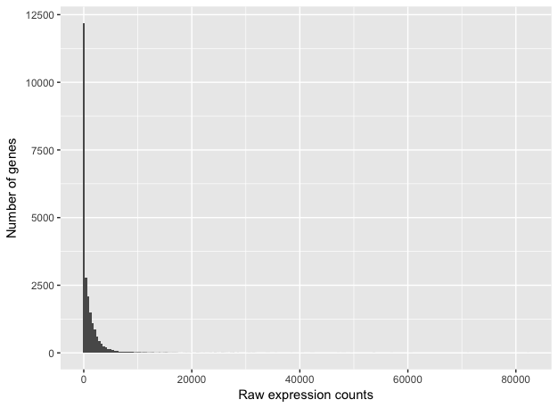
If we zoom in close to zero, we can see that there are a large number of genes with counts of zero:
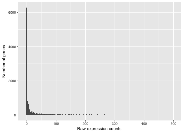
These images illustrate some common features of RNA-seq count data:
- a low number of counts associated with a large proportion of genes
- a long right tail due to the lack of any upper limit for expression
- large dynamic range
NOTE: The log intensities of the microarray data approximate a normal distribution. However, due to the different properties of the of RNA-seq count data, such as integer counts instead of continuous measurements and non-normally distributed data, the normal distribution does not accurately model RNA-seq counts [1].
Choosing an appropriate statistical model
Count data in general can be modeled with various distributions:
-
Binomial distribution: Gives you the probability of getting a number of heads upon tossing a coin a number of times. Based on discrete events and used in situations when you have a certain number of cases.
-
Poisson distribution: For use, when the number of cases is very large (i.e. people who buy lottery tickets), but the probability of an event is very small (probability of winning). The Poisson is similar to the binomial, but is based on continuous events. Appropriate for data where mean == variance.
-
Negative binomial distribution: An approximation of the Poisson, but has an additional parameter that adjusts the variance independently from the mean.
So what do we use for RNA-seq count data?
With RNA-Seq data, a very large number of RNAs are represented and the probability of pulling out a particular transcript is very small. Thus, it would be an appropriate situation to use the Poisson or Negative binomial distribution. Choosing one over the other will depend on the relationship between mean and variance in our data.
Mean versus Variance
In the figure below we have plotted the mean against the variance for three replicate samples in a study. Each data point represents a gene and the red line represents x = y.
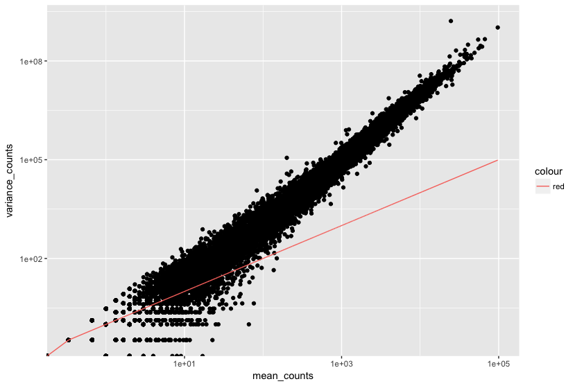
There’s two things to note here:
- The variance across replicates tends to be greater than the mean (red line), especially for genes with large mean expression levels.
- For the lowly expressed genes we see quite a bit of scatter. We usually refer to this as “heteroscedasticity”. That is, for a given expression level we observe a lot of variation in the amount of variance.
This is a good indication that our data do not fit the Poisson distribution. If the proportions of mRNA stayed exactly constant between the biological replicates for a sample group, we could expect Poisson distribution (where mean == variance). Alternatively, if we continued to add more replicates (i.e. > 20) we should eventually see the scatter start to reduce and the high expression data points move closer to the red line. So in theory, of we had enough replicates we could use the Poisson.
However, in practice a large number of replicates can be either hard to obtain (depending on how samples are obtained) and/or can be unaffordable. It is more common to see datasets with only a handful of replicates (~3-5) and reasonable amount of variation between them. The model that fits best, given this type of variability between replicates, is the Negative Binomial (NB) model. Essentially, the NB model is a good approximation for data where the mean < variance, as is the case with RNA-Seq count data.
NOTE: If we use the Poisson this will underestimate variability leading to an increase in false positive DE genes.
Tools for gene-level differential expresssion analysis
There are a number of software packages that have been developed for differential expression analysis of RNA-seq data. Many studies describing comparisons between these methods show that while there is some concordance in the genes that are identified as differentially expressed, there is also much variability between tools. Additionally, there is no one method that performs optimally under all conditions (Soneson and Dleorenzi, 2013).
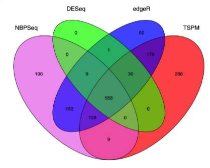
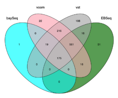
Even as new methods are continuously being developed, there are a select few that are generally recommended as best practice. Here, we list and describe three of those: DESeq2, edgeR and Limma-voom.
DESeq2 and EdgeR both use the negative binomial model, employ similar methods, and typically, yield similar results. They are both pretty stringent, and have a good balance between sensitivity and specificity (reducing both false positives and false negatives). DESeq2 does have soem extra features which implement various levels of filtering and shrinkage of fold changes to account for the heteroscedasticity described above.
Limma-Voom is another set of tools often used together for DE analysis. The Limma package was initially developed for mircroarray data where data is normally distributed. The voom functionality was introduced more recently to allow for the analysis of RNA-seq count data. Essentially weights are computed and applied to the count matrix, transforming data such that it is normally distributed and Limma functions can be applied. bThis method can be less sensitive for small sample sizes, and is recommended when the number of biological replicates per group grows large (> 20).
Tools for transcript-level differential expression analysis
Until this point we have focused on looking for expression changes at the gene-level. If you are interested in looking at splice isoform expression changes between groups, not that the previous methods (i.e DESeq2) will not work. To demonstrate how to identify transcript-level differential expression we will describe a tool called Sleuth.
Sleuth is a fast, lightweight tool that uses transcript abundance estimates output from pseudo-alignment algorithms that use bootstrap sampling, such as Sailfish, Salmon, and Kallisto, to perform differential expression analysis of gene isoforms. Sleuth accounts for this technical variability by using bootstraps as a proxy for technical replicates, which are used to model the technical variability in the abundance estimates. Bootstrapping essentially calculates the abundance estimates for all genes using a different sub-sample of reads during each round of bootstrapping. The variation in the abundance estimates output from each round of bootstrapping is used for the estimation of the technical variance for each gene.
More information about the theory/process for sleuth is available in the Nature Methods paper, this blogpost and step-by-step tutorials are available on the sleuth website.
NOTE: Kallisto is distributed under a non-commercial license, while Sailfish and Salmon are distributed under the GNU General Public License, version 3.
Hypothesis testing
With differential expression analysis, we are looking for genes/transcripts that change in expression between two or more groups, for example:
- case vs. control
- treated vs. untreated
- series of time points
Why does it not work to identify differentially expressed genes by ranking the genes by how different they are between the two groups (based on fold change values)?
Because, more often than not there is much more going on with your data than what you are anticipating. The goal of differential expression analysis to determine the relative role of these effects, and to separate the “interesting” from the “uninteresting”.
For each gene, we are assessing whether the differences in expression (counts) between groups is significant given the amount of variation observed within groups (replicates).
First, for each gene we set up a null hypothesis, which in our case is that there is no differential expression across the two sample groups. Notice that we can do this without observing any data, because it is based on a thought experiment. Second, we use a statistical test to determine if based on the observed data, the null hypothesis is true.
Pairwise comparisons using the Wald test
For RNA-seq, the Wald test is commonly used for hypothesis testing when comparing two groups. Based on the model fit (taking into account the “uninteresting” the best we can), coefficients are estimated for each gene/transcript and are used to test differences between two groups. A Wald test statistic is computed along with a probability that a test statistic at least as extreme as the observed value were selected at random. This probability is called the p-value of the test. If the p-value is small we reject the null hypothesis and state that there is evidence against the null (i.e. the gene is differentially expressed).
Likelihood Ratio Test (LRT) for multiple levels/time series
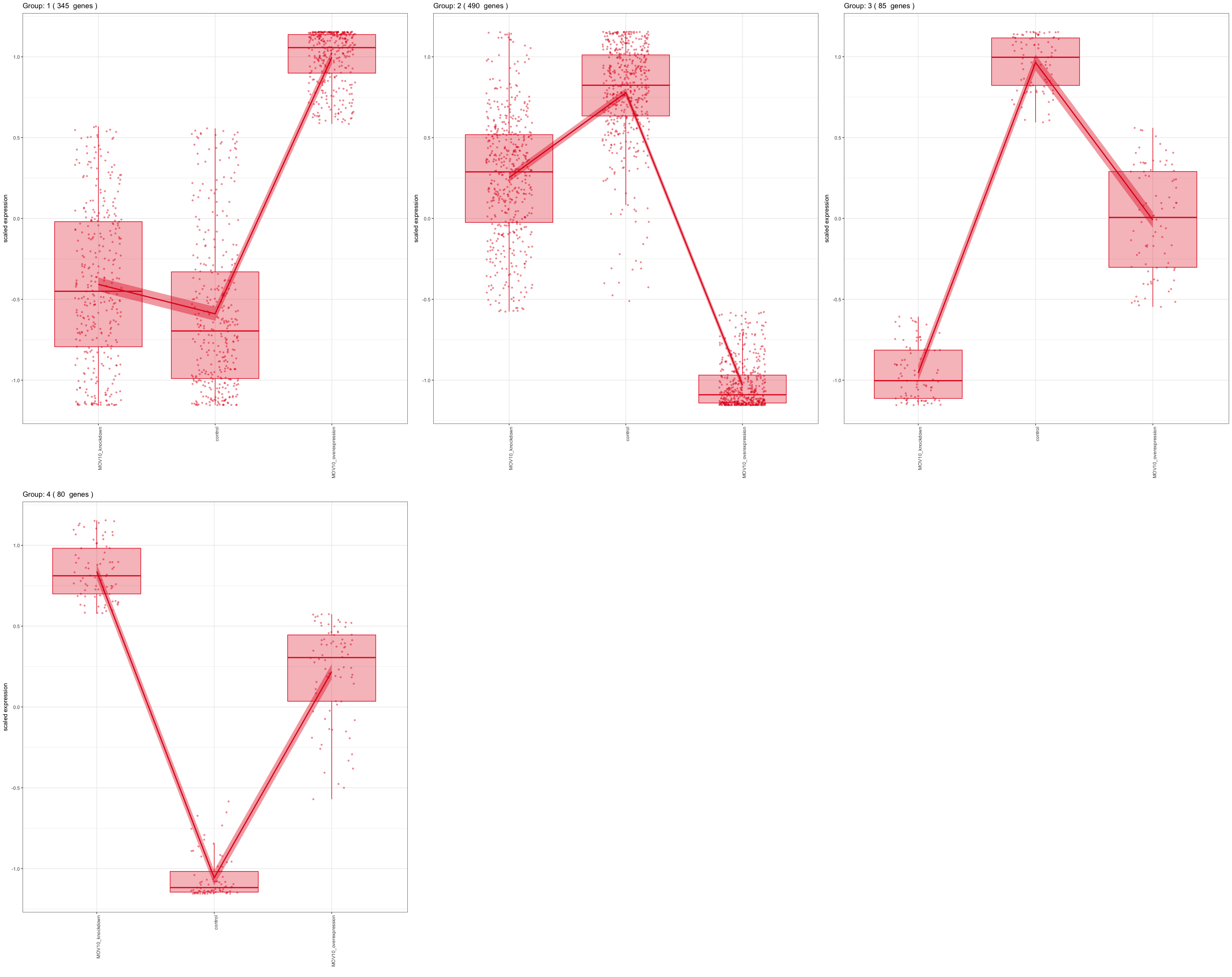
For experimental designs in which you have more than two sample groups, other statistical tests exist. For these types of comparisons, we are interested in identifying genes that show any expression change across the sample groups that we are investigating. Once we have identified those significant genes, post-hoc clustering can be applied to find groups of genes that share similar expression profiles.
In the DESeq2 package, the Likelihood Ratio Test (LRT) is implemented for the analayis of data in which there are more than two sample groups. This type of test can be especially useful in analyzing time course experiments. The LRT requires the user to identify a full model (the main effect plus all covariates) and a reduced model (the full mode without the main effect variable). The full model is then compared to the reduced model using and Analysis of Deviance (ANODEV), which is essentially testing whether the term(s) removed in the ‘reduced’ model explains a significant amount of variation in the data.
NOTE: Generally, this test will result in a larger number of genes than the individual pair-wise comparisons. While the LRT is a test of significance for differences of any level of the factor, one should not expect it to be exactly equal to the union of sets of genes using Wald tests (although we do expect a majority overlap).
Multiple test correction
From a statistical point of view, for each gene we are testing the null hypothesis that there is no differential expression across the sample groups. This may represent thousands of tests. The more genes we test, the more we inflate the false positive rate. This is the multiple testing problem.
For example, the p-value with a significance cut-off of 0.05 means there is a 5% chance of error. If we test 20,000 genes for differential expression, at p < 0.05 we would expect to find 1,000 genes by chance. If we found 3000 genes to be differentially expressed total, roughly one third of our genes are false positives. We would not want to sift through our “significant” genes to identify which ones are true positives.
There are a few commonly used approaches to correcting for this problem:
- Bonferroni: The adjusted p-value is calculated by: p-value * m (m = total number of tests). This is a very conservative approach with a high probability of false negatives, so is generally not recommended.
- FDR/Benjamini-Hochberg: Benjamini and Hochberg (1995) defined the concept of FDR and created an algorithm to control the expected FDR below a specified level given a list of independent p-values. An interpretation of the BH method for controlling the FDR is implemented in DESeq2 in which we rank the genes by p-value, then multiply each ranked p-value by m/rank.
- Q-value / Storey method: The minimum FDR that can be attained when calling that feature significant. For example, if gene X has a q-value of 0.013 it means that 1.3% of genes that show p-values at least as small as gene X are false positives
So what does FDR < 0.05 mean? The most commonly used method is the FDR. By setting the FDR cutoff to < 0.05, we’re saying that the proportion of false positives we expect amongst our differentially expressed genes is 5%. For example, if you call 500 genes as differentially expressed with an FDR cutoff of 0.05, you expect 25 of them to be false positives.
This lesson has been developed by members of the teaching team at the Harvard Chan Bioinformatics Core (HBC). These are open access materials distributed under the terms of the Creative Commons Attribution license (CC BY 4.0), which permits unrestricted use, distribution, and reproduction in any medium, provided the original author and source are credited.