Approximate time: 60 minutes
Learning Objectives
- Understanding the different steps in a differential expression analysis in the context of DESeq2
- Executing the differential expression analysis workflow with DESeq2
- Constructing design formulas appropriate for a given experimental design
- Exploring the importance of dispersion during differential expression analysis, and using the plots of the dispersion values to explore assumptions of the NB model
Differential expression analysis with DESeq2
The final step in the differential expression analysis workflow is fitting the raw counts to the NB model and performing the statistical test for differentially expressed genes. In this step we essentially want to determine whether the mean expression levels of different sample groups are significantly different.
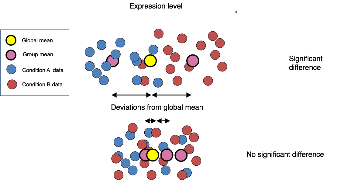
Image credit: Paul Pavlidis, UBC
The DESeq2 paper was published in 2014, but the package is continually updated and available for use in R through Bioconductor. It builds on good ideas for dispersion estimation and use of Generalized Linear Models from the DSS and edgeR methods.
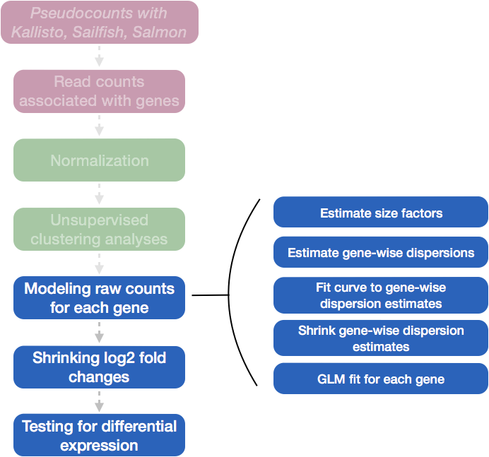
Differential expression analysis with DESeq2 involves multiple steps as displayed in the flowchart below in blue. Briefly, DESeq2 will model the raw counts, using normalization factors (size factors) to account for differences in library depth. Then, it will estimate the gene-wise dispersions and shrink these estimates to generate more accurate estimates of dispersion to model the counts. Finally, DESeq2 will fit the negative binomial model and perform hypothesis testing using the Wald test or Likelihood Ratio Test.
NOTE: DESeq2 is actively maintained by the developers and continuously being updated. As such, it is important that you note the version you are working with. Recently, there have been some rather big changes implemented that impact the output. To find out more detail about the specific modifications made to methods described in the original 2014 paper, take a look at this section in the DESeq2 vignette.
Additional details on the statistical concepts underlying DESeq2 are elucidated nicely in Rafael Irizarry’s materials for the EdX course, “Data Analysis for the Life Sciences Series”.
Running DESeq2
Prior to performing the differential expression analysis, it is a good idea to know what sources of variation are present in your data, either by exploration during the QC and/or prior knowledge. Once you know the major sources of variation, you can remove them prior to analysis or control for them in the statistical model by including them in your design formula.
Design formula
A design formula tells the statistical software the known sources of variation to control for, as well as, the factor of interest to test for during differential expression testing. For example, if you know that sex is a significant source of variation in your data, then sex should be included in your model. The design formula should have all of the factors in your metadata that account for major sources of variation in your data. The last factor entered in the formula should be the condition of interest.
For example, suppose you have the following metadata:
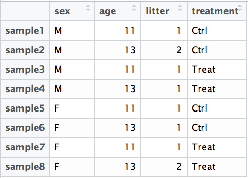
If you want to examine the expression differences between treatments, and you know that major sources of variation include sex and age, then your design formula would be:
design <- ~ sex + age + treatment
The tilde (~) should always proceed your factors and tells DESeq2 to model the counts using the following formula. Note the factors included in the design formula need to match the column names in the metadata.
Exercises
- Suppose you wanted to study the expression differences between the two age groups in the metadata shown above, and major sources of variation were
sexandtreatment, how would the design formula be written? - Based on our Mov10
metadatadataframe, which factors could we include in our design formula? - What would you do if you wanted to include a factor in your design formula that is not in your metadata?
Complex designs
DESeq2 also allows for the analysis of complex designs. You can explore interactions or ‘the difference of differences’ by specifying for it in the design formula. For example, if you wanted to explore the effect of sex on the treatment effect, you could specify for it in the design formula as follows:
design <- ~ sex + age + treatment + sex:treatment
Since the interaction term sex:treatment is last in the formula, the results output from DESeq2 will output results for this term.
There are additional recommendations for complex designs in the DESeq2 vignette. In addition, Limma documentation offers additional insight into creating more complex design formulas.
NOTE: Need help figuring out what information should be present in your metadata? We have additional materials highlighting bulk RNA-seq planning considerations. Please take a look at these materials before starting an experiment to help with proper experimental design.
MOV10 DE analysis
Now that we know how to specify the model to DESeq2, we can run the differential expression pipeline on the raw counts.
To get our differential expression results from our raw count data, we only need to run 2 lines of code!
First we create a DESeqDataSet as we did in the ‘Count normalization’ lesson and specify the txi object which contains our raw counts, the metadata variable, and provide our design formula:
## Create DESeq2Dataset object
dds <- DESeqDataSetFromTximport(txi, colData = meta, design = ~ sampletype)
Then, to run the actual differential expression analysis, we use a single call to the function DESeq().
## Run analysis
dds <- DESeq(dds)
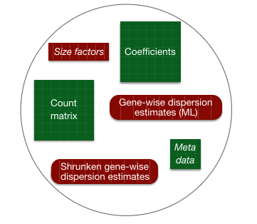
By re-assigning the results of the function back to the same variable name (dds), we can fill in the slots of our DESeqDataSet object.
Everything from normalization to linear modeling was carried out by the use of a single function! This function will print out a message for the various steps it performs:
estimating size factors
estimating dispersions
gene-wise dispersion estimates
mean-dispersion relationship
final dispersion estimates
fitting model and testing
NOTE: There are individual functions available in DESeq2 that would allow us to carry out each step in the workflow in a step-wise manner, rather than a single call. We demonstrated one example when generating size factors to create a normalized matrix. By calling
DESeq(), the individual functions for each step are run for you.
DESeq2 differential gene expression analysis workflow
With the 2 lines of code above, we just completed the workflow for the differential gene expression analysis with DESeq2. The steps in the analysis are output below:
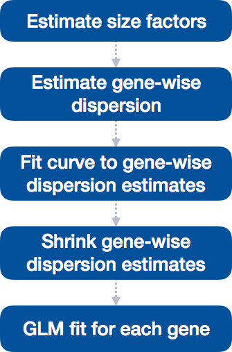
We will be taking a detailed look at each of these steps to better understand how DESeq2 is performing the statistical analysis and what metrics we should examine to explore the quality of our analysis.
Step 1: Estimate size factors
The first step in the differential expression analysis is to estimate the size factors, which is exactly what we already did to normalize the raw counts.
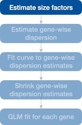
DESeq2 will automatically estimate the size factors when performing the differential expression analysis. However, if you have already generated the size factors using estimateSizeFactors(), as we did earlier, then DESeq2 will use these values.
To normalize the count data, DESeq2 calculates size factors for each sample using the median of ratios method discussed previously in the ‘Count normalization’ lesson.
MOV10 DE analysis: examining the size factors
Let’s take a quick look at size factor values we have for each sample:
## Check the size factors
sizeFactors(dds)

Irrel_kd_1 Irrel_kd_2 Irrel_kd_3 Mov10_kd_2 Mov10_kd_3 Mov10_oe_1 Mov10_oe_2
 1.1149694  0.9606733  0.7492240  1.5633640  0.9359695  1.2262649  1.1405026
Mov10_oe_3
 0.6542030
These numbers should be identical to those we generated initially when we had run the function estimateSizeFactors(dds). Take a look at the total number of reads for each sample:
## Total number of raw counts per sample
colSums(counts(dds))
How do the numbers correlate with the size factor?
Now take a look at the total depth after normalization using:
## Total number of normalized counts per sample
colSums(counts(dds, normalized=T))
How do the values across samples compare with the total counts taken for each sample?
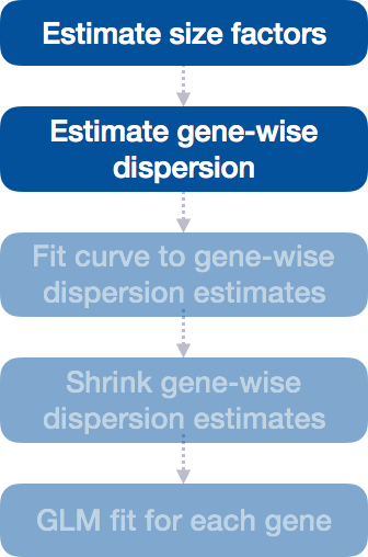
Step 2: Estimate gene-wise dispersion
The next step in the differential expression analysis is the estimation of gene-wise dispersions. Before we get into the details, we should have a good idea about what dispersion is referring to in DESeq2.
In RNA-seq count data, we know:
- To determine differentially expressed genes, we need to identify genes that have significantly different mean expression between groups given the variation within the groups (between replicates).
- The variation within group (between replicates) needs to account for the fact that variance increases with the mean expression, as shown in the plot below (each black dot is a gene).
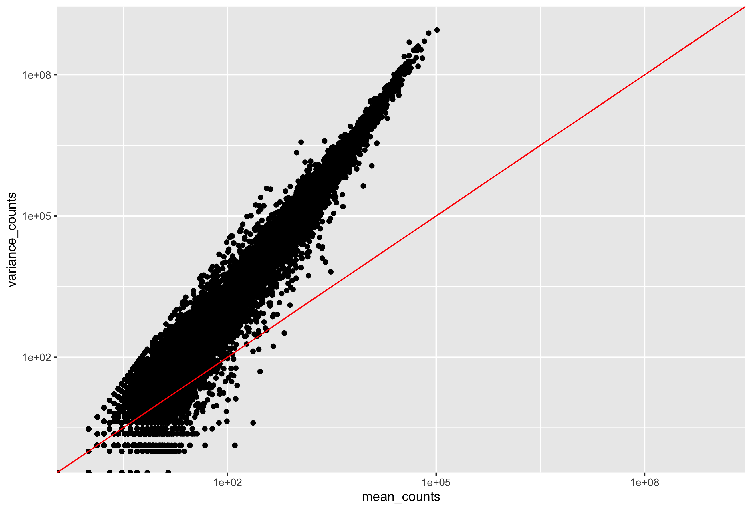
To accurately identify DE genes, DESeq2 needs to account for the relationship between the variance and mean. We don’t want all of our DE genes to be genes with low counts because the variance is lower for lowly expressed genes.
Instead of using variance as the measure of variation in the data (since variance correlates with gene expression level), it uses a measure of variation called dispersion, which accounts for a gene’s variance and mean expression level. Dispersion is calculated by Var = μ + α*μ^2, where α represents the dispersion (Var = variance, and μ = mean) giving the relationship:
| Effect on dispersion | |
|---|---|
| Variance increases | Dispersion increases |
| Mean expression increases | Dispersion decreases |
For genes with moderate to high count values, the square root of dispersion will be equal to the coefficient of variation (Var / μ). So 0.01 dispersion means 10% variation around the mean expected across biological replicates. The dispersion estimates for genes with the same mean will differ only based on their variance. Therefore, the dispersion estimates reflect the variance in gene expression for a given mean value (given as black dots in image below).
How does the dispersion relate to our model?
To accurately model sequencing counts, we need to generate accurate estimates of within-group variation (variation between replicates of the same sample group) for each gene. With only a few (3-6) replicates per group, the estimates of variation for each gene are often unreliable.
To address this problem, DESeq2 shares information across genes to generate more accurate estimates of variation based on the mean expression level of the gene using a method called ‘shrinkage’. DESeq2 assumes that genes with similar expression levels have similar dispersion.
Estimating the dispersion for each gene separately:
DESeq2 estimates the dispersion for each gene based on the gene’s expression level (mean counts of replicates) and variance.
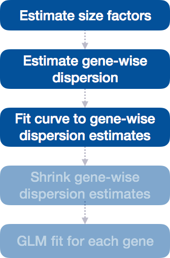
Step 3: Fit curve to gene-wise dispersion estimates
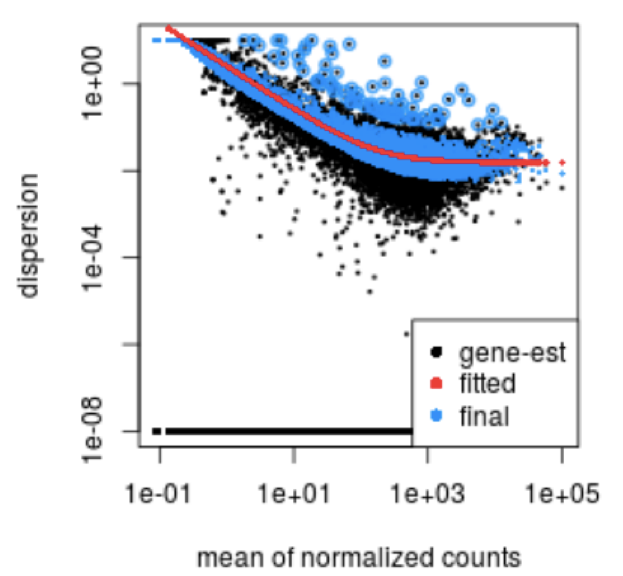
The next step in the workflow is to fit a curve to the gene-wise dispersion estimates. The idea behind fitting a curve to the data is that different genes will have different scales of biological variability, but, across all genes, there will be a distribution of reasonable estimates of dispersion.
This curve is displayed as a red line in the figure below, which plots the estimate for the expected dispersion value for genes of a given expression strength. Each black dot is a gene with an associated mean expression level and maximum likelihood estimation (MLE) of the dispersion (Step 1).
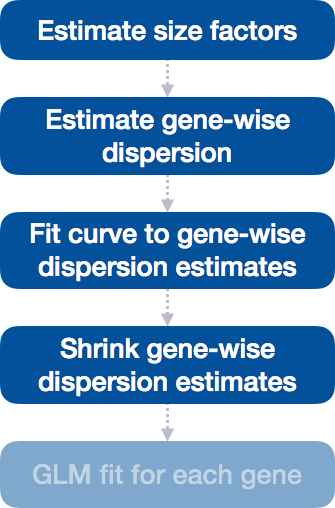
Step 4: Shrink gene-wise dispersion estimates toward the values predicted by the curve
The next step in the workflow is to shrink the gene-wise dispersion estimates toward the expected dispersion values.
The curve allows for more accurate identification of differentially expressed genes when sample sizes are small, and the strength of the shrinkage for each gene depends on :
- how close gene dispersions are from the curve
- sample size (more samples = less shrinkage)
This shrinkage method is particularly important to reduce false positives in the differential expression analysis. Genes with low dispersion estimates are shrunken towards the curve, and the more accurate, higher shrunken values are output for fitting of the model and differential expression testing.
Dispersion estimates that are slightly above the curve are also shrunk toward the curve for better dispersion estimation; however, genes with extremely high dispersion values are not. This is due to the likelihood that the gene does not follow the modeling assumptions and has higher variability than others for biological or technical reasons [1]. Shrinking the values toward the curve could result in false positives, so these values are not shrunken. These genes are shown surrounded by blue circles below.
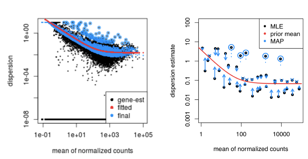
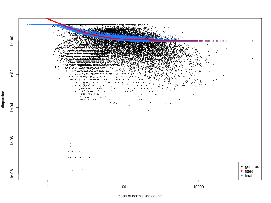
This is a good plot to examine to ensure your data is a good fit for the DESeq2 model. You expect your data to generally scatter around the curve, with the dispersion decreasing with increasing mean expression levels. If you see a cloud or different shapes, then you might want to explore your data more to see if you have contamination (mitochondrial, etc.) or outlier samples. Note how much shrinkage you get across the whole range of means in the plotDispEsts() plot for any experiment with low degrees of freedom.
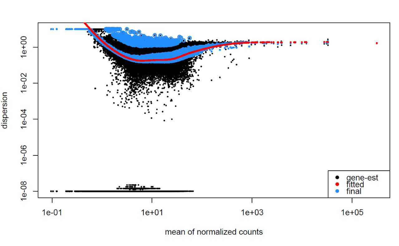
Examples of worrisome dispersion plots are shown below:
MOV10 DE analysis: exploring the dispersion estimates and assessing model fit
Let’s take a look at the dispersion estimates for our MOV10 data:
## Plot dispersion estimates
plotDispEsts(dds)
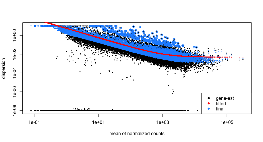
Since we have a small sample size, for many genes we see quite a bit of shrinkage. Do you think our data are a good fit for the model?
This lesson has been developed by members of the teaching team at the Harvard Chan Bioinformatics Core (HBC). These are open access materials distributed under the terms of the Creative Commons Attribution license (CC BY 4.0), which permits unrestricted use, distribution, and reproduction in any medium, provided the original author and source are credited.
Some materials and hands-on activities were adapted from RNA-seq workflow on the Bioconductor website