Approximate time: 60 minutes
Learning Objectives
- Introducing an alternative statistical test for differential expression analysis
- Extract results using the LRT and compare to Wald test
- Export results to file
Hypothesis testing: Likelihood ratio test (LRT)
An alternative to pair-wise comparisons is to analyze all levels of a factor at once. By default the Wald test is used to generate the results table, but DESeq2 also offers the LRT which is used to identify any genes that show change in expression across the different levels. This type of test can be especially useful in analyzing time course experiments.
To use the LRT, we use the DESeq() function but this time adding two arguments:
- specifying that we want to use the LRT test
- the ‘reduced’ model
library(DESeq2)
library(DEGreport)

# The full model was specified previously with the `design = ~ sampletype`:
# dds <- DESeqDataSetFromMatrix(countData = data, colData = meta, design = ~ sampletype)

# Likelihood ratio test
dds_lrt <- DESeq(dds, test="LRT", reduced = ~ 1)
Since our ‘full’ model only has one factor (sampletype), the ‘reduced’ model is just the intercept.
The LRT is comparing the full model to the reduced model to identify significant genes. The p-values are determined solely by the difference in deviance between the ‘full’ and ‘reduced’ model formula (not log2 fold changes). Essentially the LRT test is testing whether the term(s) removed in the ‘reduced’ model explains a significant amount of variation in the data?
Generally, this test will result in a larger number of genes than the individual pair-wise comparisons. While the LRT is a test of significance for differences of any level of the factor, one should not expect it to be exactly equal to the union of sets of genes using Wald tests (although we do expect a majority overlap).
Let’s take a look at the results table:
# Extract results
res_LRT <- results(dds_lrt)
You will find that similar columns are reported for the LRT test. One thing to note is, even though there are fold changes present they are not directly associated with the actual hypothesis test. Thus, when filtering significant genes from the LRT we use only the FDR as our threshold. How many genes are significant at padj < 0.05?
# Subset the LRT results to return genes with padj < 0.05
sig_res_LRT <- res_LRT %>%
               data.frame() %>%
               rownames_to_column(var="gene") %>%
               as_tibble() %>%
               filter(padj < padj.cutoff)

# Get sig gene lists
sigLRT_genes <- sig_res_LRT %>%
                pull(gene)

length(sigLRT_genes)

# Compare to numbers we had from Wald test
nrow(sigOE)
nrow(sigKD)
How many genes from the Mov10 overexpression Wald test are contained in the LRT gene set? And for the Mov10 knockdown?
The number of significant genes observed from the LRT is quite high. We are unable to set a fold change criteria here since the statistic is not generated from any one pairwise comparison. This list includes genes that can be changing in any number of combinations across the three factor levels. It is advisable to instead increase the stringency on our criteria and lower the FDR threshold.
Exercise
- Using a more stringent cutoff of
padj < 0.001, count how many genes are significant using the LRT method. - Set the variables
OEgenesandKDgenesto contain the genes that meet the thresholdpadj < 0.001. - Find the overlapping number of genes between these gene sets and the genes from LRT at
padj < 0.001.
Identifying gene clusters exhibiting particular patterns across samples
Often we are interested in genes that have particular patterns across the sample groups (levels) of our condition. For example, with the MOV10 dataset, we may be interested in genes that exhibit the lowest expression for the Mov10_KD and highest expression for the Mov10_OE sample groups (i.e. KD < CTL < OE). To identify genes associated with these patterns we can use a clustering tool, degPatterns from the ‘DEGreport’ package, that groups the genes based on their changes in expression across sample groups.
First we will subset our rlog transformed normalized counts to contain only the differentially expressed genes (padj < 0.05).
# Subset results for faster cluster finding (for classroom demo purposes)
clustering_sig_genes <- sig_res_LRT %>%
                  arrange(padj) %>%
                  head(n=1000)


# Obtain rlog values for those significant genes
cluster_rlog <- rld_mat[clustering_sig_genes$gene, ]
Then we can use the degPatterns function from the ‘DEGreport’ package to determine sets of genes that exhibit similar expression patterns across sample groups. The degPatterns tool uses a hierarchical clustering approach based on pair-wise correlations, then cuts the hierarchical tree to generate groups of genes with similar expression profiles. The tool cuts the tree in a way to optimize the diversity of the clusters, such that the variability inter-cluster > the variability intra-cluster.
# Use the `degPatterns` function from the 'DEGreport' package to show gene clusters across sample groups
clusters <- degPatterns(cluster_rlog, metadata = meta, time = "sampletype", col=NULL)
Let’s explore the output:
# What type of data structure is the `clusters` output?
class(clusters)

# Let's see what is stored in the `df` component
head(clusters$df)
While we don’t see any clusters with the pattern we are looking for (KD < CTL < OE), we do see a lot of genes that don’t change much between control and knockdown sample groups, but increase drastically with the overexpression group (Group 1).
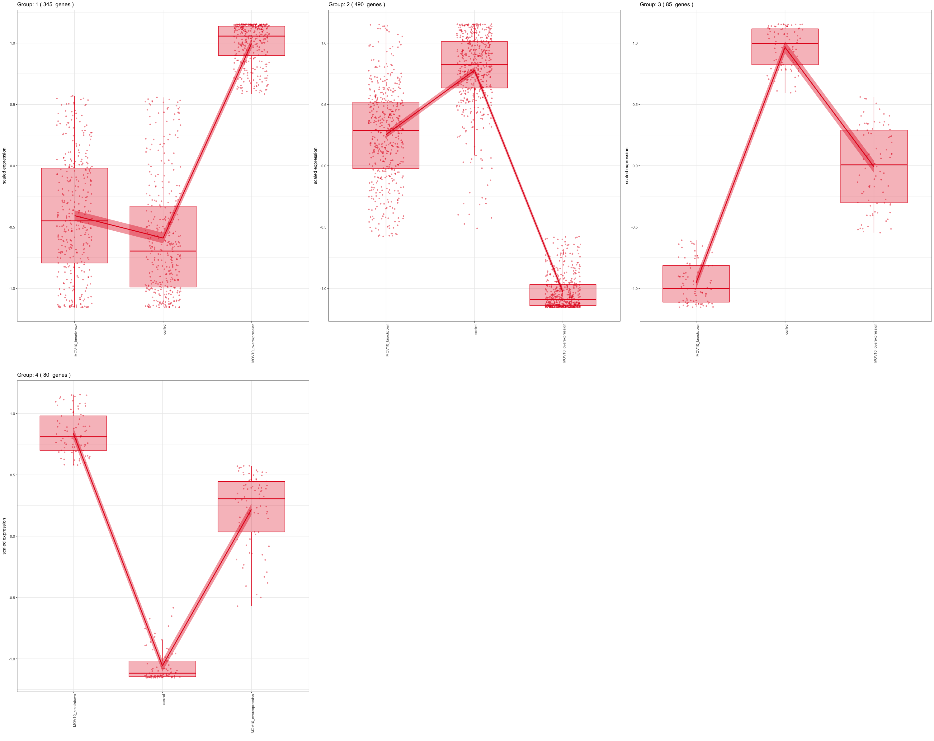
Let’s explore the set of genes in Group 1 in more detail:
# Extract the Group 1 genes
cluster_groups <- clusters$df
group1 <- clusters$df %>%
          filter(cluster == 1)
After extracting a group of genes, we can perform functional analysis to explore associated functions. We can repeat this extraction and functional analysis for any of the groups of interest.
Time course analyses with LRT
The LRT test can be especially helpful when performing time course analyses. We can use the LRT to explore whether there are any significant differences in treatment effect between any of the timepoints.
For have an experiment looking at the effect of treatment over time on mice of two different genotypes. We could use a design formula for our ‘full model’ that would include the major sources of variation in our data: genotype, treatment, time, and our main condition of interest, which is the difference in the effect of treatment over time (treatment:time).
full_model <- ~ genotype + treatment + time + treatment:time
To perform the LRT test, we can determine all genes that have significant differences in expression between treatments across time points by giving the ‘reduced model’ without the treatment:time term:
reduced_model <- ~ genotype + treatment + time
Then, we could run our test by using the following code:
dds <- DESeqDataSetFromMatrix(countData = raw_counts, colData = metadata, design = ~ genotype + treatment + time + treatment:time)

dds_lrt_time <- DESeq(dds, test="LRT", reduced = ~ genotype + treatment + time)
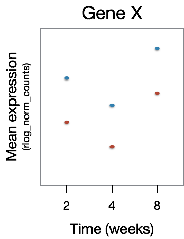
This analysis will not return genes where the treatment effect does not change over time, even though the genes may be differentially expressed between groups at a particular time point, as shown in the figure below:
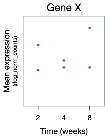
The significant DE genes will represent those genes that have differences in the effect of treatment over time, an example is displayed in the figure below:
Once we have our results, we can determine the significant genes using a threshold of padj < 0.05 and return the normalized counts for those genes. Then we could perform clustering to identify genes that change over time in a way meaningful to us:
clusters <- degPatterns(cluster_rlog, metadata = meta, time="time", col="treatment")
You can extract the groups of genes associated with the patterns of interest similar to the actions performed previously, then move on to functional analysis for each of the gene groups of interest.
Resources
We have covered the inner workings of DESeq2 in a fair amount of detail such that when using this package you have a good understanding of what is going on under the hood. For more information on topics covered, we encourage you to take a look at the following resources:
- DESeq2 vignette
- GitHub book on RNA-seq gene level analysis
- Bioconductor support site (posts tagged with
deseq2)
This lesson has been developed by members of the teaching team at the Harvard Chan Bioinformatics Core (HBC). These are open access materials distributed under the terms of the Creative Commons Attribution license (CC BY 4.0), which permits unrestricted use, distribution, and reproduction in any medium, provided the original author and source are credited.
- Materials and hands-on activities were adapted from RNA-seq workflow on the Bioconductor website