Approximate time: 60 minutes
Learning Objectives
- Understanding the different steps in a differential expression analysis in the context of DESeq2
- Building results tables for comparison of different sample classes
- Summarizing significant differentially expressed genes for each comparison
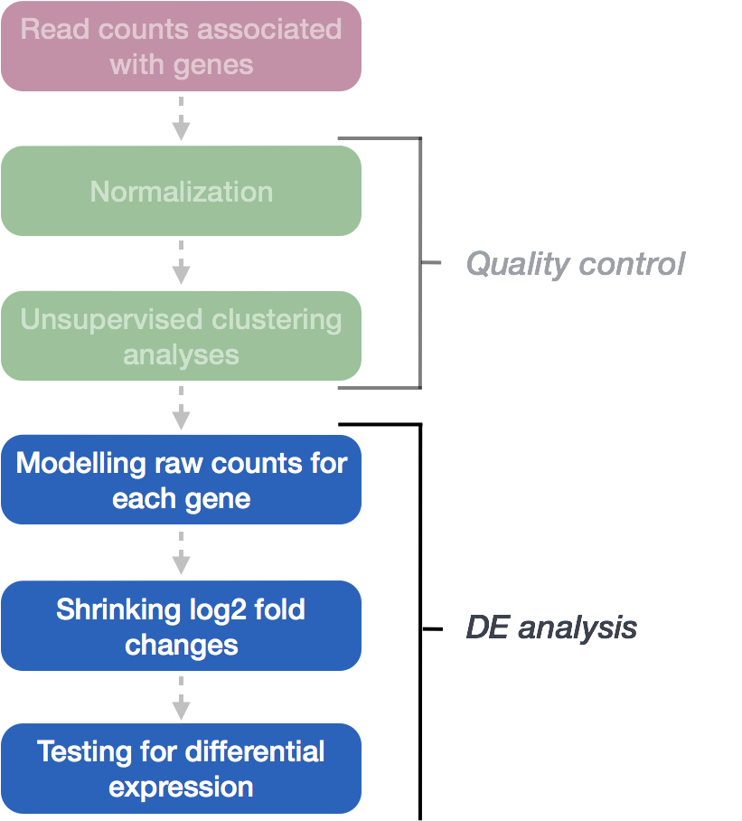
Differential expression analysis with DESeq2: model fitting and hypothesis testing
Generalized Linear Model fit for each gene
The final step in the DESeq2 workflow is fitting the Negative Binomial model for each gene and performing differential expression testing.
As discussed earlier, the count data generated by RNA-seq exhibits overdispersion (variance > mean) and the statistical distribution used to model the counts needs to account for this overdispersion. DESeq2 uses a negative binomial distribution to model the RNA-seq counts using the equation below:
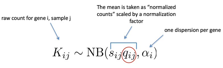
Modeling is a mathematically formalized way to approximate how the data behaves given a set of parameters (i.e. size factor, dispersion). DESeq2 will use this formula as our model for each gene, and fit the normalized count data to it. After the model is fit, coefficients are estimated for each sample group along with their standard error using the formula:
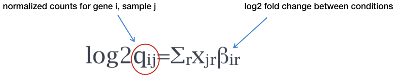
The coefficents are the estimates for the log2 foldchanges for each sample group. However, these estimates do not account for the large dispersion we observe with low read counts. To avoid this, the log2 fold changes calculated by the model need to be adjusted.
Shrunken log2 foldchanges (LFC)
To generate more accurate log2 foldchange estimates, DESeq2 allows for the shrinkage of the LFC estimates toward zero when the information for a gene is low, which could include:
- Low counts
- High dispersion values
As with the shrinkage of dispersion estimates, LFC shrinkage uses information from all genes to generate more accurate estimates. Specifically, the distribution of LFC estimates for all genes is used (as a prior) to shrink the LFC estimates of genes with little information or high dispersion toward more likely (lower) LFC estimates.
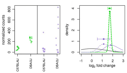
Illustration taken from the DESeq2 paper.
For example, in the figure above, the green gene and purple gene have the same mean values for the two sample groups (C57BL/6J and DBA/2J), but the green gene has little variation while the purple gene has high levels of variation. For the green gene with low variation, the unshrunken LFC estimate (vertex of the green solid line) is very similar to the shrunken LFC estimate (vertex of the green dotted line), but the LFC estimates for the purple gene are quite different due to the high dispersion. So even though two genes can have similar normalized count values, they can have differing degrees of LFC shrinkage. Notice the LFC estimates are shrunken toward the prior (black solid line).
In the most recent versions of DESeq2, the shrinkage of LFC estimates is not performed by default. This means that the log2 foldchanges would be the same as those calculated by:
log2 (normalized_counts_group1 / normalized_counts_group2)
To generate the shrunken log2 fold change estimates, you have to run an additional step on your results object (that we will create below) with the function lfcShrink().
NOTE: Shrinking the log2 fold changes will not change the total number of genes that are identified as significantly differentially expressed. The shrinkage of fold change is to help with downstream assessment of results. For example, if you wanted to subset your significant genes based on fold change for further evaluation, you may want to use shruken values. Additionally, for functional analysis tools such as GSEA which require fold change values as input you would want to provide shrunken values.
NOTE: Older versions of DESeq2 (< 1.16.0) shrink the fold changes by default, so if you are using an older version of the tool and very large expected fold changes for a number of individual genes are expected, but not enough such that the prior would not include such large fold changes, then you may want to turn off LFC shrinkage.
For these older versions of DESeq2, you can turn off the beta prior when calling the
DESeq()function:DESeq(dds, betaPrior=FALSE). By turning off the prior, the log2 foldchanges would be the same as those calculated by:
log2 (normalized_counts_group1 / normalized_counts_group2)
Hypothesis testing using the Wald test
The first step in hypothesis testing is to set up a null hypothesis for each gene. In our case is, the null hypothesis is that there is no differential expression across the two sample groups (LFC == 0). Notice that we can do this without observing any data, because it is based on a thought experiment. Second, we use a statistical test to determine if based on the observed data, the null hypothesis is true.
With DESeq2, the Wald test is commonly used for hypothesis testing when comparing two groups. A Wald test statistic is computed along with a probability that a test statistic at least as extreme as the observed value were selected at random. This probability is called the p-value of the test. If the p-value is small we reject the null hypothesis and state that there is evidence against the null (i.e. the gene is differentially expressed).
Creating contrasts
To indicate to DESeq2 the two groups we want to compare, we can use contrasts. Contrasts are then provided to DESeq2 to perform differential expression testing using the Wald test. Contrasts can be provided to DESeq2 a couple of different ways:
- Do nothing. Automatically DESeq2 will use the base factor level of the condition of interest as the base for statistical testing. The base level is chosen based on alphabetical order of the levels.
-
In the
results()function you can specify the comparison of interest, and the levels to compare. The level given last is the base level for the comparison. The syntax is given below:# DO NOT RUN! contrast <- c("condition", "level_to_compare", "base_level") results(dds, contrast = contrast, alpha = alpha_threshold)NOTE: The Wald test can also be used with continuous variables. If the variable of interest provided in the design formula is continuous-valued, then the reported log2 fold change is per unit of change of that variable.
MOV10 DE analysis: contrasts and Wald tests
We have three sample classes so we can make three possible pairwise comparisons:
- Control vs. Mov10 overexpression
- Control vs. Mov10 knockdown
- Mov10 knockdown vs. Mov10 overexpression
We are really only interested in #1 and #2 from above. Using the design formula we provided ~ sampletype, indicating that this is our main factor of interest.
Building the results table
To build our results table we will use the results() function. To tell DESeq2 which groups we wish to compare, we supply the contrasts we would like to make using thecontrast argument. For this example we will save the unshrunken and shrunken versions of results to separate variables. Additionally, we are including the alpha argument and setting it to 0.05. This is the significance cutoff used for optimizing the independent filtering (by default it is set to 0.1). If the adjusted p-value cutoff (FDR) will be a value other than 0.1 (for our final list of significant genes), alpha should be set to that value.
## Define contrasts, extract results table, and shrink the log2 fold changes

contrast_oe <- c("sampletype", "MOV10_overexpression", "control")

res_tableOE_unshrunken <- results(dds, contrast=contrast_oe, alpha = 0.05)

res_tableOE <- lfcShrink(dds, contrast=contrast_oe, res=res_tableOE_unshrunken)
The order of the names determines the direction of fold change that is reported. The name provided in the second element is the level that is used as baseline. So for example, if we observe a log2 fold change of -2 this would mean the gene expression is lower in Mov10_oe relative to the control.
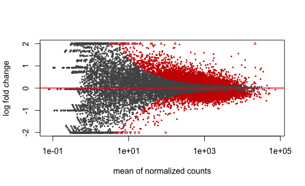
MA Plot
A plot that can be useful to exploring our results is the MA plot. The MA plot shows the mean of the normalized counts versus the log2 foldchanges for all genes tested. The genes that are significantly DE are colored to be easily identified. This is also a great way to illustrate the effect of LFC shrinkage. The DESeq2 package offers a simple function to generate an MA plot.
Let’s start with the unshrunken results:
plotMA(res_tableOE_unshrunken, ylim=c(-2,2))
And now the shrunken results:
plotMA(res_tableOE, ylim=c(-2,2))
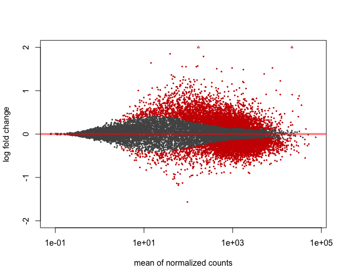
In addition to the comparison described above, this plot allows us to evaluate the magnitude of fold changes and how they are distributed relative to mean expression. Generally, we would expect to see significant genes across the full range of expression levels.
MOV10 DE analysis: results exploration
The results table looks very much like a dataframe and in many ways it can be treated like one (i.e when accessing/subsetting data). However, it is important to recognize that it is actually stored in a DESeqResults object. When we start visualizing our data, this information will be helpful.
class(res_tableOE)
Let’s go through some of the columns in the results table to get a better idea of what we are looking at. To extract information regarding the meaning of each column we can use mcols():
mcols(res_tableOE, use.names=T)
baseMean: mean of normalized counts for all sampleslog2FoldChange: log2 fold changelfcSE: standard errorstat: Wald statisticpvalue: Wald test p-valuepadj: BH adjusted p-values
Now let’s take a look at what information is stored in the results:
res_tableOE %>% data.frame() %>% View()
log2 fold change (MAP): sampletype MOV10_overexpression vs control
Wald test p-value: sampletype MOV10_overexpression vs control
DataFrame with 6 rows and 6 columns
               baseMean log2FoldChange      lfcSE       stat    pvalue       padj
              <numeric>      <numeric>  <numeric>  <numeric> <numeric>  <numeric>
1/2-SBSRNA4  45.6520399     0.26976764 0.18775752  1.4367874 0.1507784 0.25242910
A1BG         61.0931017     0.20999700 0.17315013  1.2128030 0.2252051 0.34444163
A1BG-AS1    175.6658069    -0.05197768 0.12366259 -0.4203185 0.6742528 0.77216278
A1CF          0.2376919     0.02237286 0.04577046  0.4888056 0.6249793         NA
A2LD1        89.6179845     0.34598540 0.15901426  2.1758136 0.0295692 0.06725157
A2M           5.8600841    -0.27850841 0.18051805 -1.5428286 0.1228724 0.21489067
NOTE: on p-values set to NA
- If within a row, all samples have zero counts, the baseMean column will be zero, and the log2 fold change estimates, p-value and adjusted p-value will all be set to NA.
- If a row contains a sample with an extreme count outlier then the p-value and adjusted p-value will be set to NA. These outlier counts are detected by Cook’s distance.
- If a row is filtered by automatic independent filtering, for having a low mean normalized count, then only the adjusted p-value will be set to NA.
Multiple test correction
Note that we have pvalues and p-adjusted values in the output. Which should we use to identify significantly differentially expressed genes?
If we used the p-value directly from the Wald test with a significance cut-off of p < 0.05, that means there is a 5% chance it is a false positives. Each p-value is the result of a single test (single gene). The more genes we test, the more we inflate the false positive rate. This is the multiple testing problem. For example, if we test 20,000 genes for differential expression, at p < 0.05 we would expect to find 1,000 genes by chance. If we found 3000 genes to be differentially expressed total, roughly one third of our genes are false positives. We would not want to sift through our “significant” genes to identify which ones are true positives.
DESeq2 helps reduce the number of genes tested by removing those genes unlikely to be significantly DE prior to testing, such as those with low number of counts and outlier samples (gene-level QC). However, we still need to correct for multiple testing to reduce the number of false positives, and there are a few common approaches:
- Bonferroni: The adjusted p-value is calculated by: p-value * m (m = total number of tests). This is a very conservative approach with a high probability of false negatives, so is generally not recommended.
- FDR/Benjamini-Hochberg: Benjamini and Hochberg (1995) defined the concept of FDR and created an algorithm to control the expected FDR below a specified level given a list of independent p-values. An interpretation of the BH method for controlling the FDR is implemented in DESeq2 in which we rank the genes by p-value, then multiply each ranked p-value by m/rank.
- Q-value / Storey method: The minimum FDR that can be attained when calling that feature significant. For example, if gene X has a q-value of 0.013 it means that 1.3% of genes that show p-values at least as small as gene X are false positives
In DESeq2, the p-values attained by the Wald test are corrected for multiple testing using the Benjamini and Hochberg method by default. There are options to use other methods in the results() function. The p-adjusted values should be used to determine significant genes. The significant genes can be output for visualization and/or functional analysis.
So what does FDR < 0.05 mean? By setting the FDR cutoff to < 0.05, we’re saying that the proportion of false positives we expect amongst our differentially expressed genes is 5%. For example, if you call 500 genes as differentially expressed with an FDR cutoff of 0.05, you expect 25 of them to be false positives.
MOV10 DE analysis: Control versus Knockdown
Now that we have results for the overexpression results, let’s do the same for the Control vs. Knockdown samples. Use contrasts in the results() to extract a results table and store that to a variable called res_tableKD.
## Define contrasts, extract results table and shrink log2 fold changes
contrast_kd <-  c("sampletype", "MOV10_knockdown", "control")

res_tableKD <- results(dds, contrast=contrast_kd, alpha = 0.05)

res_tableKD <- lfcShrink(dds, contrast=contrast_kd, res=res_tableKD)
Take a quick peek at the results table containing Wald test statistics for the Control-Knockdown comparison we are interested in and make sure that format is similar to what we observed with the OE.
Summarizing results
To summarize the results table, a handy function in DESeq2 is summary(). Confusingly it has the same name as the function used to inspect data frames. This function when called with a DESeq results table as input, will summarize the results using the alpha threshold: FDR < 0.05 (padj/FDR is used even though the output says p-value < 0.05). Let’s start with the OE vs control results:
## Summarize results
summary(res_tableOE)
In addition to the number of genes up- and down-regulated at the default threshold, the function also reports the number of genes that were tested (genes with non-zero total read count), and the number of genes not included in multiple test correction due to a low mean count.
Extracting significant differentially expressed genes
What we noticed is that the FDR threshold on it’s own doesn’t appear to be reducing the number of significant genes. With large significant gene lists it can be hard to extract meaningful biological relevance. To help increase stringency, one can also add a fold change threshold. The summary() function doesn’t have an argument for fold change threshold.
Let’s first create variables that contain our threshold criteria:
### Set thresholds
padj.cutoff <- 0.05
lfc.cutoff <- 0.58
The lfc.cutoff is set to 0.58; remember that we are working with log2 fold changes so this translates to an actual fold change of 1.5 which is pretty reasonable.
We can easily subset the results table to only include those that are significant using the filter() function, but first we will convert the results table into a tibble:
res_tableOE_tb <- res_tableOE %>%
  data.frame() %>%
  rownames_to_column(var="gene") %>%
  as_tibble()
Now we can subset that table to only keep the significant genes using our pre-defined thresholds:
sigOE <- res_tableOE_tb %>%
        filter(padj < padj.cutoff & abs(log2FoldChange) > lfc.cutoff)
How many genes are differentially expressed in the Overexpression compared to Control, given our criteria specified above? Does this reduce our results?
sigOE
Using the same thresholds as above (padj.cutoff < 0.05 and lfc.cutoff = 0.58), subset res_tableKD to report the number of genes that are up- and down-regulated in Mov10_knockdown compared to control.
res_tableKD_tb <- res_tableKD %>%
  data.frame() %>%
  rownames_to_column(var="gene") %>%
  as_tibble()

sigKD <- res_tableKD_tb %>%
        filter(padj < padj.cutoff & abs(log2FoldChange) > lfc.cutoff)
How many genes are differentially expressed in the Knockdown compared to Control?
sigKD
Now that we have subsetted our data, we are ready for visualization!
An alternative approach
The
results()function has an option to add a fold change threshold using thelfcThrehsoldargument. This method is more statistically motivated, and is recommended when you want a more confident set of genes based on a certain fold-change. It actually performs a statistical test against the desired threshold, by performing a two-tailed test for log2 fold changes greater than the absolute value specified. The user can change the alternative hypothesis usingaltHypothesisand perform two one-tailed tests as well. This is a more conservative approach, so expect to retrieve a much smaller set of genes!Test this out using our data:
results(dds, contrast = contrast_oe, alpha = 0.05, lfcThreshold = 0.58)How do the results differ? How many significant genes do we get using this approach?
This lesson has been developed by members of the teaching team at the Harvard Chan Bioinformatics Core (HBC). These are open access materials distributed under the terms of the Creative Commons Attribution license (CC BY 4.0), which permits unrestricted use, distribution, and reproduction in any medium, provided the original author and source are credited.
Some materials and hands-on activities were adapted from RNA-seq workflow on the Bioconductor website